Amplitude-Based Circuits#
This page documents the components that are used in algorithms that use the A mplitude B ased (AB) Encoding. At the moment, this includes two algorihtms:
The “regular” Amplitude-Based Collisionless QLBM: ABQLBM,
The Multi-Speed (MS) Collisionless QLBM: MSQLBM.
ABQLBM uses ABLattices and OHLattices, while MSQLBM is built from MSLattices.
The general interface of CQLBM is built from all 3 lattice instances and delegeates to the appropriate implementation automatically.
Both algorithms are instances of the Collisionless QLBM (CQLBM), also known as the
Quantum Transport Method (QTM).
Both algorithms compress the grid and the vnumber of discrete velocities
into \(N_g\cdot N_v \mapsto \lceil \log_2 N_g \rceil + \lceil \log_2 N_v \rceil\) qubits.
The amplitude of each basis state is directly related to the populations in the classical LBM discretization.
The MSQLBM is a generalization of the ABQLBM.
The implementation of the algorithms was first described in [10] and later expanded in [11].
At its core, the CQLBM algorithm manipulates the particle probability distribution in an amplitude-based encoding of the quantum state. The End-to-end algorithms can be broken down into several distinct steps:
Initial Conditions conditions prepare the starting state of the probability distribution function.
Streaming circuits increment or decrement the position of particles in physical space through QFT-based streaming.
Reflection circuits apply boundary conditions that affect particles that come in contact with solid obstacles. Reflection places those particles back in the appropriate position of the fluid domain.
Measurement operations extract information out of the quantum state, which can later be post-processed classically.
This page documents the individual components that make up the CQLBM algorithm. Subsections follow a top-down approach, where end-to-end operators are introduced first, before being broken down into their constituent parts.
End-to-end algorithms#
- class qlbm.components.CQLBM(lattice, use_agnostic_bcs=False, logger=<Logger qlbm (WARNING)>)[source]#
The end-to-end algorithm of the Collisionless Quantum Lattice Boltzmann Algorithm first introduced in Schalkers and Möller [10] and later extended in Schalkers and Möller [11].
Implementations based on lattices with the DdQq discretization use the
ABQLBM:from qlbm.components import CQLBM from qlbm.lattice import ABLattice lattice = ABLattice( { "lattice": {"dim": {"x": 4, "y": 4}, "velocities": "d2q9"}, "geometry": [], } ) CQLBM(lattice).draw("mpl")
(
Source code,png,hires.png,pdf)
Implementations where the number of velocities is defined per dimension delegate to the
MSQLBM.from qlbm.components import CQLBM from qlbm.lattice import MSLattice lattice = MSLattice( { "lattice": {"dim": {"x": 4, "y": 4}, "velocities": {"x": 4, "y": 4}}, "geometry": [], } ) CQLBM(lattice).draw("mpl")
(
Source code,png,hires.png,pdf)
- Parameters:
lattice (Lattice)
use_agnostic_bcs (bool)
logger (Logger)
- class qlbm.components.ms.MSQLBM(lattice, group_velocities=False, logger=<Logger qlbm (WARNING)>)[source]#
The end-to-end algorithm of the Multi-Speed Collisionless Quantum Lattice Boltzmann Algorithm first introduced in Schalkers and Möller [10] and later extended in Schalkers and Möller [11].
This implementation supports 2D and 3D simulations with with cuboid objects with either bounce-back or specular reflection boundary conditions.
The algorithm is composed of three steps that are repeated according to a CFL counter:
Streaming performed by the
MSStreamingOperatorincrements or decrements the positions of particles on the grid.BounceBackReflectionOperatorandSpecularReflectionOperatorreflect the particles that come in contact withBlockobstacles encoded in theMSLattice.The
StreamingAncillaPreparationresets the state of the ancilla qubits for the next CFL counter substep.
Attribute
Summary
latticeThe
MSLatticebased on which the properties of the operator are inferred.loggerThe performance logger, by default
getLogger("qlbm").group_velocitiesWhether to group velocities into 1 streaming step in the CFL series.
- Parameters:
lattice (Lattice)
group_velocities (bool)
logger (Logger)
- class qlbm.components.ab.ABQLBM(lattice, use_agnostic_bcs=False, logger=<Logger qlbm (WARNING)>)[source]#
Implementation of the A mplitude B ased QLBM (ABQLBM).
The algorithm consists of interleaving steps of streaming and boundary conditions. Note that there is no collision in this algorithm as of yet. Details of the general framework can be found in [10]. The ABQLBM works with \(D_dQ_q\) discretizations only. For multi-speed alternatives, see
MSQLBM.Eample usage:
from qlbm.components.ab import ABQLBM
from qlbm.lattice import ABLattice

# Example with streaming only for simplicity.
lattice = ABLattice(
    {
        "lattice": {"dim": {"x": 16, "y": 8}, "velocities": "d2q9"},
        "geometry": [],
    }
)

ABQLBM(lattice).draw("mpl")
- Parameters:
lattice (Lattice)
use_agnostic_bcs (bool)
logger (Logger)
Initial Conditions#
- class qlbm.components.ms.primitives.MSInitialConditions(lattice, logger=<Logger qlbm (WARNING)>)[source]#
A primitive that creates the quantum circuit to prepare the flow field in its initial conditions for the
MSLattice.The initial conditions create a quantum state spanning half the grid in the x-axis, and the entirety of the y (and z)-axes (if 3D). All velocities are pointing in the positive direction.
Attribute
Summary
latticeThe
MSLatticebased on which the properties of the operator are inferred.loggerThe performance logger, by default
getLogger("qlbm").Example usage:
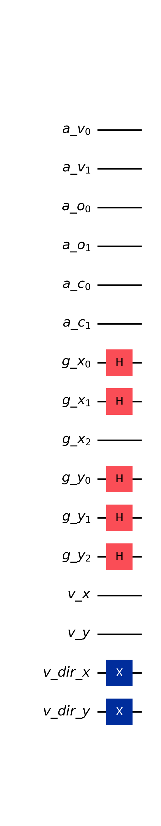
from qlbm.components.ms import MSInitialConditions
from qlbm.lattice import MSLattice

# Build an example lattice
lattice = MSLattice({
    "lattice": {
        "dim": {
                "x": 8,
                "y": 8
            },
            "velocities": {
                "x": 4,
                "y": 4
        }
    },
    "geometry": [
        {
            "shape": "cuboid",
            "x": [5, 6],
            "y": [1, 2],
            "boundary": "specular"
        }
    ]
})

# Draw the initial conditions circuit
MSInitialConditions(lattice).draw("mpl")
(
Source code,png,hires.png,pdf)
- Parameters:
lattice (MSLattice)
logger (Logger)
- class qlbm.components.ms.primitives.MSInitialConditions3DSlim(lattice, logger=<Logger qlbm (WARNING)>)[source]#
A primitive that creates the quantum circuit to prepare the flow field in its initial conditions for 3 dimensions.
The initial conditions create the quantum state \(\Sigma_{j}\ket{0}^{\otimes n_{g_x}}\ket{0}^{\otimes n_{g_y}}\ket{j}\) over the grid qubits, that is, spanning the z-axis at the bottom of the x- and y-axes. This is helpful for debugging edge cases around the corners of 3D obstacles. All velocities are pointing in the positive direction.
Attribute
Summary
latticeThe
MSLatticebased on which the properties of the operator are inferred.loggerThe performance logger, by default
getLogger("qlbm").Example usage:
from qlbm.components.ms import MSInitialConditions3DSlim
from qlbm.lattice import MSLattice

# Build an example lattice
lattice = MSLattice({
    "lattice": {
        "dim": {
        "x": 8,
        "y": 8,
        "z": 8
        },
        "velocities": {
        "x": 4,
        "y": 4,
        "z": 4
        }
    },
    "geometry": []
})

# Draw the initial conditions circuit
MSInitialConditions3DSlim(lattice).draw("mpl")
(
Source code,png,hires.png,pdf)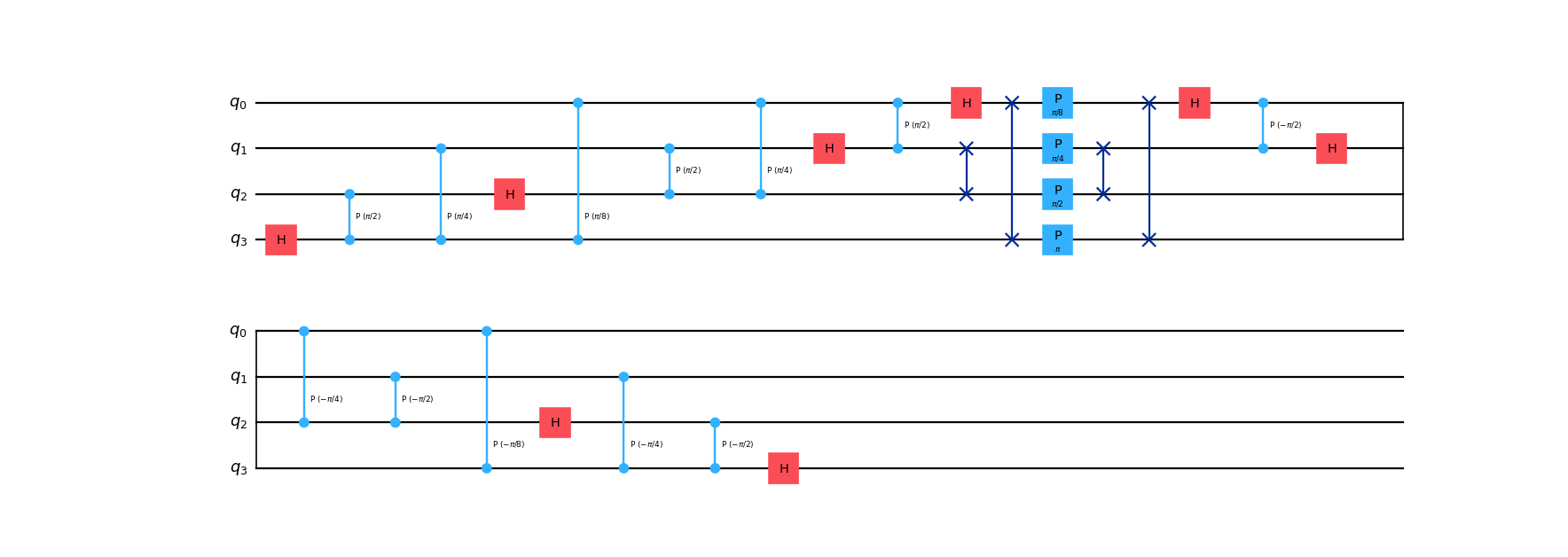
- Parameters:
lattice (MSLattice)
logger (Logger)
- class qlbm.components.ab.initial.ABDiscreteUniformInitialConditions(lattice, velocity_indices, grid_qubits_to_superpose, logger=<Logger qlbm (WARNING)>)[source]#
Initial conditions for the
ABQLBMalgorithm.This component creates an equal magnitude superposition of a configurable set of velocity and grid indices.
Example usage:
from qlbm.components.ab import ABDiscreteUniformInitialConditions
from qlbm.lattice import ABLattice

lattice = ABLattice(
    {
        "lattice": {"dim": {"x": 16, "y": 8}, "velocities": "d2q9"},
    }
)

ABDiscreteUniformInitialConditions(lattice, [1, 3, 4], ([], [])).draw("mpl")
(
Source code,png,hires.png,pdf)
The primitive can also applied to the
OHLattice:from qlbm.components.ab import ABDiscreteUniformInitialConditions from qlbm.lattice import OHLattice lattice = OHLattice( { "lattice": {"dim": {"x": 16, "y": 8}, "velocities": "d2q9"}, } ) ABDiscreteUniformInitialConditions(lattice, [0, 1], ([0, 1], [0])).draw("mpl")
(
Source code,png,hires.png,pdf)
- Parameters:
lattice (ABLattice)
velocity_indices (List[int])
grid_qubits_to_superpose (Tuple[List[int], ...])
logger (Logger)
- class qlbm.components.ab.initial.ABParallelDiscreteUniformInitialConditions(lattice, velocity_indices_list, grid_qubits_to_superpose_list, logger=<Logger qlbm (WARNING)>)[source]#
Marker-sensitive initial conditions for the
ABQLBMalgorithm.This component creates an equal magnitude superposition of a configurable set of velocity and grid indices, entangled with the state of the marker register. Used in parallel realizations of configurations.
Example usage:
from qlbm.components.ab import ABParallelDiscreteUniformInitialConditions
from qlbm.lattice import ABLattice

lattice = ABLattice(
    {
        "lattice": {"dim": {"x": 16, "y": 8}, "velocities": "d2q9"},
    }
)

lattice.set_num_marker_qubits(2)

ABParallelDiscreteUniformInitialConditions(
    lattice,
    [[0, 1], [0, 3], [0], [0, 5]],
    [([0], [0])] * 4,
).draw("mpl")
(
Source code,png,hires.png,pdf)
- Parameters:
lattice (ABLattice)
velocity_indices_list (List[List[int]])
grid_qubits_to_superpose_list (List[Tuple[List[int], ...]])
logger (Logger)
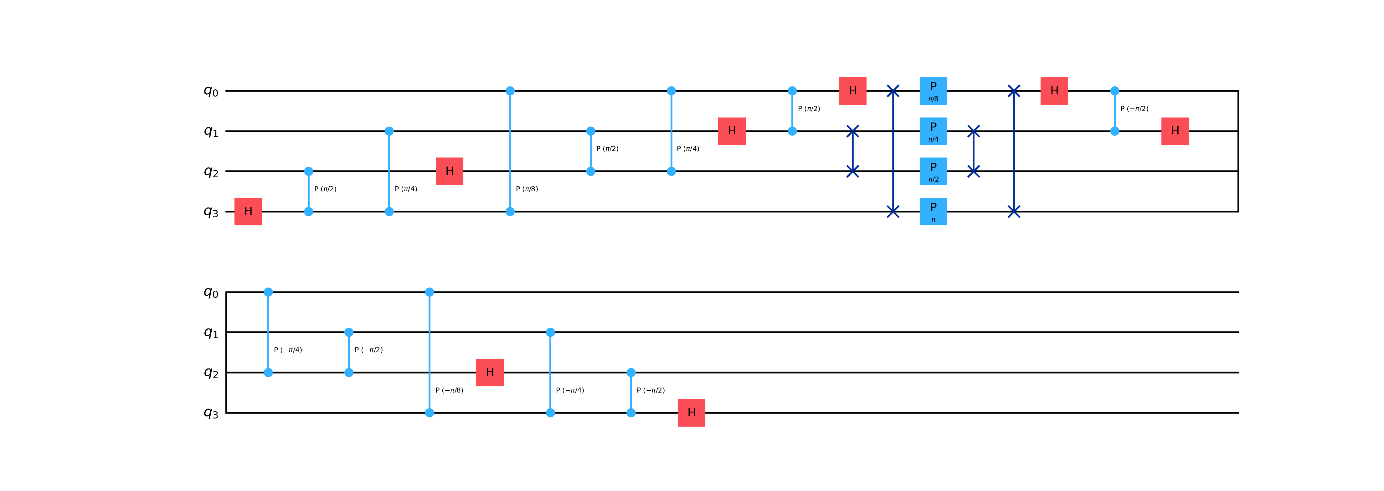
- class qlbm.components.ab.initial.ABInitialConditions(lattice, logger=<Logger qlbm (WARNING)>)[source]#
Initial conditions for the
ABQLBMalgorithm.This component creates an equal magnitude superposition of all velocity basis states at position
(0, 0)using theUniformStatePrep.Example usage:
from qlbm.components.ab import ABInitialConditions
from qlbm.lattice import ABLattice

lattice = ABLattice(
    {
        "lattice": {"dim": {"x": 16, "y": 8}, "velocities": "d2q9"},
        "geometry": [],
    }
)

ABInitialConditions(lattice).draw("mpl")
(
Source code,png,hires.png,pdf)
You can also get the low-level decomposition of the circuit as:
from qlbm.components.ab import ABInitialConditions
from qlbm.lattice import ABLattice

lattice = ABLattice(
    {
        "lattice": {"dim": {"x": 4, "y": 4}, "velocities": "d2q9"},
        "geometry": [],
    }
)

ABInitialConditions(lattice).circuit.decompose(reps=2).draw("mpl")
(
Source code,png,hires.png,pdf)
- Parameters:
lattice (ABLattice)
logger (Logger)
Streaming#
- class qlbm.components.ms.streaming.MSStreamingOperator(lattice, velocities, logger=<Logger qlbm (WARNING)>)[source]#
An operator that performs streaming in Fourier space as part of the
MSQLBMalgorithm.Streaming is broken down into the following steps:
A
StreamingAncillaPreparationobject prepares the ancilla velocity qubits for CFL time step. This happens independently for all dimensions, and it is assumed the velocity discretization is uniform across dimensions.A
ControlledIncrementerperforms incrementation or decrementation in the Fourier space, controlled on the ancilla qubits set in the previous steps.For efficiency reasons, the velocity qubits set in step 1 are not reset, as they will be re-used in the subsequent reflection step. Another instance of the
StreamingAncillaPreparationwould be required to consistently end the step.
For an in-depth mathematical explanation of the procedure, consult Section 4 of Schalkers and Möller [10].
Attribute
Summary
latticeThe
MSLatticebased on which the properties of the operator are inferred.velocitiesA list of velocities to increment. This is computed according to CFL counter.
loggerThe performance logger, by default
getLogger("qlbm").Example usage:
from qlbm.components.ms import MSStreamingOperator
from qlbm.lattice import MSLattice

# Build an example lattice
lattice = MSLattice(
    {
        "lattice": {"dim": {"x": 8, "y": 8}, "velocities": {"x": 4, "y": 4}},
        "geometry": [],
    }
)

# Streaming the velocity with index 2
MSStreamingOperator(lattice=lattice, velocities=[2]).draw("mpl")
(
Source code,png,hires.png,pdf)
- Parameters:
lattice (MSLattice)
velocities (List[int])
logger (Logger)
- class qlbm.components.ms.streaming.StreamingAncillaPreparation(lattice, velocities, dim, logger=<Logger qlbm (WARNING)>)[source]#
A primitive used in
MSStreamingOperatorthat implements the preparatory step of streaming necessary for theMSQLBMmethod.This operator sets the ancilla qubits to \(\ket{1}\) for the velocities that will be streamed in the next CFL time step.
Attribute
Summary
latticeThe
MSLatticebased on which the properties of the operator are inferred.velocitiesThe velocities that need to be streamed within the next time step.
dimThe dimension to which the velocities correspond.
loggerThe performance logger, by default
getLogger("qlbm").Example usage:
from qlbm.components.ms import StreamingAncillaPreparation
from qlbm.lattice import MSLattice

# Build an example lattice
lattice = MSLattice(
    {
        "lattice": {"dim": {"x": 8, "y": 8}, "velocities": {"x": 4, "y": 4}},
        "geometry": [],
    }
)

# Streaming velocities indexed 2 in the y (1) dimension
StreamingAncillaPreparation(lattice=lattice, velocities=[2], dim=1).draw("mpl")
(
Source code,png,hires.png,pdf)
- Parameters:
lattice (MSLattice)
velocities (List[int])
dim (int)
logger (Logger)
- class qlbm.components.ms.streaming.ControlledIncrementer(lattice, reflection=None, logger=<Logger qlbm (WARNING)>)[source]#
A primitive used in
MSStreamingOperatorthat implements the streaming operation on the states for which the ancilla qubits are in the state \(\ket{1}\).This primitive is applied after the primitive
StreamingAncillaPreparationto compose the streaming operator.Attribute
Summary
latticeThe
MSLatticebased on which the properties of the operator are inferred.reflectionThe reflection attribute decides the type of reflection that will take place. This should be either “specular”, “bounceback”, or
None, and defaults to None. This parameter governs which qubits are used as controls for the Fourier space phase shifts.loggerThe performance logger, by default
getLogger("qlbm").Example usage:
from qlbm.components.ms import ControlledIncrementer
from qlbm.lattice import MSLattice

# Build an example lattice
lattice = MSLattice(
    {
        "lattice": {"dim": {"x": 8, "y": 8}, "velocities": {"x": 4, "y": 4}},
        "geometry": [],
    }
)

# Streaming velocities indexed 2 in the y (1) dimension
ControlledIncrementer(lattice=lattice).draw("mpl")
(
Source code,png,hires.png,pdf)
- Parameters:
lattice (MSLattice)
reflection (str | None)
logger (Logger)
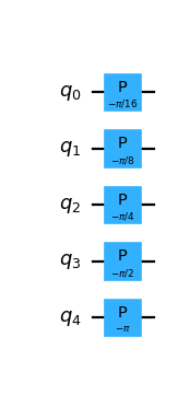
- class qlbm.components.ms.streaming.PhaseShift(num_qubits, positive=False, logger=<Logger qlbm (WARNING)>)[source]#
A primitive that applies the phase-shift as part of the
ControlledIncrementerused in theMSStreamingOperator.The rotation applied is \(\pm\frac{\pi}{2^{n_q - 1 - j}}\), with \(j\) the position of the qubit (indexed starting with 0). For an in-depth mathematical explanation of the procedure and its use within QLBM, consult Section 4 of Schalkers and Möller [10]. The Draper adder was originally formulated in [2], while the version implemented here uses the one-register approach, which was first described in [1].
Attribute
Summary
num_qubitsThe number of qubits to perform the phase shift for.
positiveWhether the phase shift is applied to increment (T) or decrement (F) the position of the particles. Defaults to
False.loggerThe performance logger, by default
getLogger("qlbm").Example usage:
from qlbm.components.common.adders import PhaseShift

# A phase shift of 5 qubits
PhaseShift(num_qubits=5, positive=False).draw("mpl")
(
Source code,png,hires.png,pdf)
- Parameters:
num_qubits (int)
positive (bool)
logger (Logger)
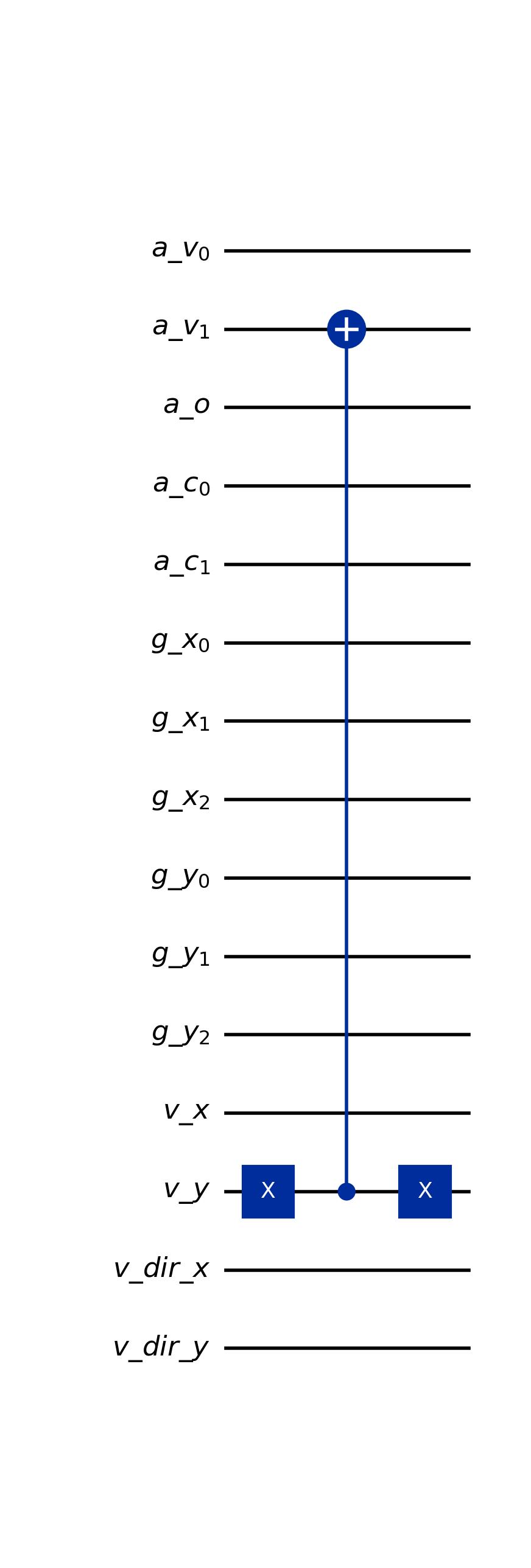
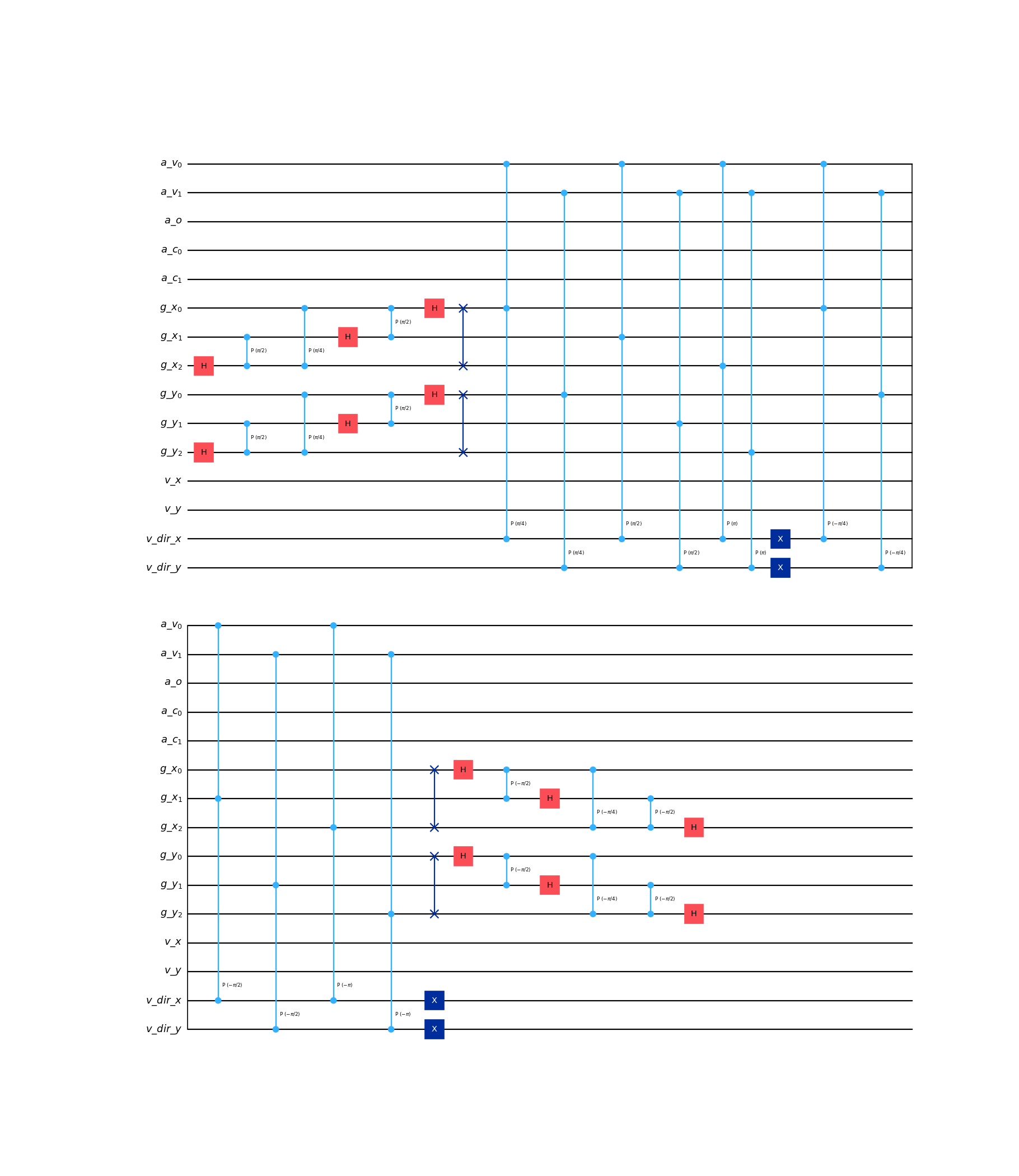
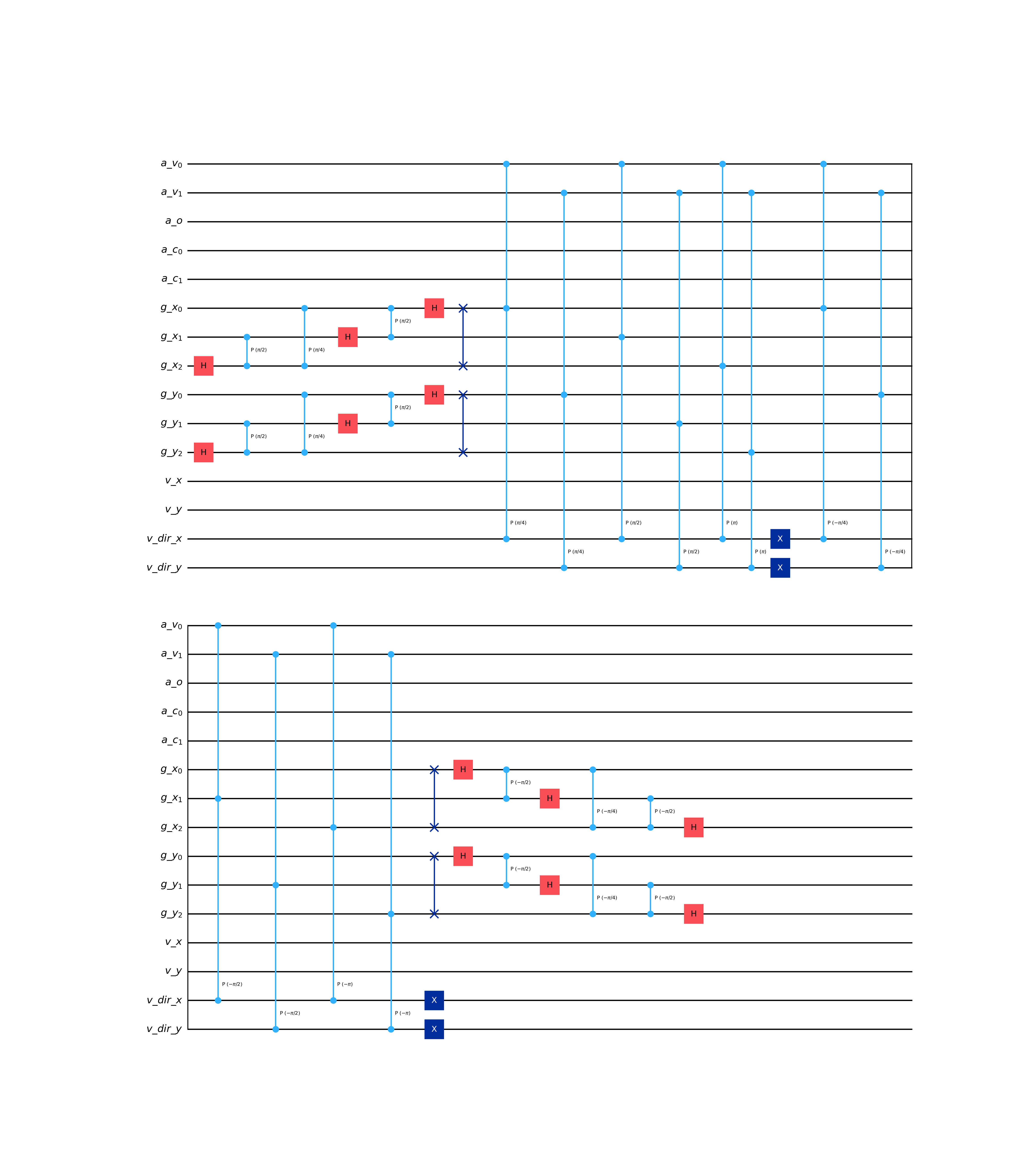
- class qlbm.components.ab.streaming.ABStreamingOperator(lattice, additional_control_qubit_indices=[], logger=<Logger qlbm (WARNING)>)[source]#
Streaming operator for the
ABQLBMalgorithm.Uses a variant of the Draper adder described in [10]. The operator works by applying QFTs in parallel to each dimension of the grid, followed by phase gates that perform incrementation in the Fourier basis, and, finally, by applying an inverse QFT mapping the qubits back to the computational basis.
Populations are streamed one after the other in Fourier space by controlling phase gates on the state of the velocity qubits. Additional controls qubits can be specified to restrict this operation.
Example usage:
from qlbm.components.ab import ABStreamingOperator
from qlbm.lattice import ABLattice

lattice = ABLattice(
    {
        "lattice": {"dim": {"x": 4, "y": 8}, "velocities": "d2q9"},
        "geometry": [],
    }
)

ABStreamingOperator(lattice).draw("mpl")
(
Source code,png,hires.png,pdf)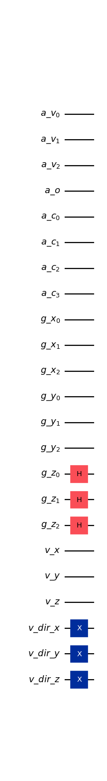
- Parameters:
lattice (AmplitudeLattice)
additional_control_qubit_indices (List[int])
logger (Logger)
Reflection#
- class qlbm.components.ms.bounceback_reflection.BounceBackReflectionOperator(lattice, blocks, logger=<Logger qlbm (WARNING)>)[source]#
Operator implementing the 2D and 3D Bounce-Back (BB) boundary conditions as described in Schalkers and Möller [11].
The operator parses information encoded in
Blockobjects to detect particles that have virtually streamed into the solid domain before placing them back to their previous positions in the fluid domain. The pseudocode for this procedure is as follows:Components of the quantum state that encode particles that have streamed inside the obstacle are identified with
BounceBackWallComparatorobjects;These components have their velocity direction qubits flipped in all three dimensions;
Particles are streamed outside the solid domain with inverted velocity directions;
Once streamed outside the solid domain, components encoding affected particles have their obstacle ancilla qubit reset based on grid position, velocity direction, and whether they have streamed in the CFL timestep.
Attribute
Summary
latticeThe
MSLatticebased on which the properties of the operator are inferred.blocksA list of
Blockobjects for which to generate the BB boundary condition circuits.loggerThe performance logger, by default
getLogger("qlbm").Example usage:
from qlbm.components.ms import BounceBackReflectionOperator
from qlbm.lattice import MSLattice

# Build an example lattice
lattice = MSLattice(
    {
        "lattice": {"dim": {"x": 8, "y": 8}, "velocities": {"x": 4, "y": 4}},
        "geometry": [{"shape":"cuboid", "x": [5, 6], "y": [1, 2], "boundary": "bounceback"}],
    }
)

BounceBackReflectionOperator(lattice=lattice, blocks=lattice.shape_list)
- create_circuit()[source]#
Creates the
qiskit.QuantumCircuitof this object.This method is called automatically at construction time for all quantum components.
- Returns:
The generated QuantumCircuit.
- Return type:
QuantumCircuit
- reflect_wall(circuit, wall)[source]#
Performs reflection based on information encoded in a
ReflectionWallas follows.A series of \(X\) gates set the grid qubits to the \(\ket{1}\) state for the dimension that the wall spans.
Comparator circuits set the comparator ancilla qubits to \(\ket{1}\) based on the size of the wall in the other dimension(s).
Depending on the use, the directional velocity qubits are also set to \(\ket{1}\) based on the dimension that the wall spans.
A multi-controlled \(X\) gate flips the obstacle ancilla qubit, controlled on the qubits set in the previous steps.
The control qubits are set back to their previous state.
The wall reflection operation is versatile and can be used to both set and re-set the state of the obstacle ancilla qubit at different stages of reflection. When performing BB reflection, this function is first used to flip the ancilla obstacle qubit from \(\ket{0}\) to \(\ket{1}\), irrespective of how particles arrived there. Subsequently, an additional controls are placed on the velocity direction qubits to reset the ancilla obstacle qubit to \(\ket{0}\), after particles have been streamed out of the solid domain.
- Parameters:
circuit (QuantumCircuit) – The circuit on which to perform BB reflection of the wall.
wall (ReflectionWall) – The wall encoding the reflection logic.
inside_obstacle (bool) – Whether the wall is inside the obstacle.
- Returns:
The circuit performing BB reflection of the wall.
- Return type:
QuantumCircuit
- reset_edge_state(circuit, edge)[source]#
Resets the state of an edge along the side of an obstacle in 3D as follows.
A series of \(X\) gates set the grid qubits to the \(\ket{1}\) state for the 2 dimensions that the edge spans.
A comparator circuits sets the comparator ancilla qubits to \(\ket{1}\) based on the size of the edge in the remaining dimension.
The directional velocity qubits are also set to \(\ket{1}\) on the specific velocity profile of the targeted particles.
A multi-controlled \(X\) gate flips the obstacle ancilla qubit, controlled on the qubits set in the previous steps.
The control qubits are set back to their previous state.
This function resets the ancilla obstacle qubit to \(\ket{0}\) for particles along 36 specific edges of a cube after those particles have been streamed out of the obstacle in the CFL time step.
- Parameters:
circuit (QuantumCircuit) – The circuit on which to perform resetting of the edge state.
edge (ReflectionResetEdge) – The edge on which to apply the reflection reset logic.
- Returns:
The circuit performing the resetting of the edge state.
- Return type:
QuantumCircuit
- reset_point_state(circuit, corner)[source]#
Resets the state of the ancilla obstacle qubit of a single point on the grid as follows.
A series of \(X\) gates set the grid qubits to the \(\ket{1}\) state for the dimension that the wall spans.
The directional velocity qubits are also set to \(\ket{1}\) based on the specific velocity profile of the targeted particles.
A multi-controlled \(X\) gate flips the obstacle ancilla qubit, controlled on the qubits set in the previous steps.
The control qubits are set back to their previous state.
- Parameters:
circuit (QuantumCircuit) – The circuit on which to perform the resetting of the point state.
corner (ReflectionPoint) – The corner for which to reset the desired point states.
- Returns:
The circuit resetting the point state as desired.
- Return type:
QuantumCircuit
- flip_and_stream(circuit)[source]#
Flips the velocity direction qubit controlled on the ancilla obstacle qubit, before performing streaming.
Unlike in the regular
MSStreamingOperator, theControlledIncrementerphase shift circuit is additionally controlled on the ancilla obstacle qubit, which ensures that only particles whose grid position gets incremented (decremented) are those that have streamed inside the solid domain in this CFL time step.- Parameters:
circuit (QuantumCircuit) – The circuit on which to perform the flip and stream operation.
- class qlbm.components.ms.specular_reflection.SpecularReflectionOperator(lattice, blocks, logger=<Logger qlbm (WARNING)>)[source]#
Operator implementing the 2D and 3D Specular Reflection (SR) boundary conditions as described Schalkers and Möller [10].
The operator parses information encoded in
Blockobjects to detect particles that have virtually streamed into the solid domain before placing them back to their previous positions in the fluid domain. The pseudocode for this procedure is as follows:Components of the quantum state that encode particles that have streamed inside the obstacle are identified with
SpecularWallComparatorobjects;These components have their velocity direction qubits flipped according to the wall they came in contact with. Where two or three walls come together, the two or three corresponding directions are inverted;
Particles are streamed outside the solid domain with inverted velocity directions;
Once streamed outside the solid domain, components encoding affected particles have their obstacle ancilla qubits reset based on grid position, velocity direction, and whether they have streamed in the CFL timestep.
Attribute
Summary
latticeThe
MSLatticebased on which the properties of the operator are inferred.blocksA list of
Blockobjects for which to generate the BB boundary condition circuits.loggerThe performance logger, by default
getLogger("qlbm").Example usage:
from qlbm.components.ms import SpecularReflectionOperator
from qlbm.lattice import MSLattice

# Build an example lattice
lattice = MSLattice(
    {
        "lattice": {"dim": {"x": 8, "y": 8}, "velocities": {"x": 4, "y": 4}},
        "geometry": [{"shape":"cuboid", "x": [5, 6], "y": [1, 2], "boundary": "specular"}],
    }
)

SpecularReflectionOperator(lattice=lattice, blocks=lattice.shape_list)
- create_circuit()[source]#
Creates the
qiskit.QuantumCircuitof this object.This method is called automatically at construction time for all quantum components.
- Returns:
The generated QuantumCircuit.
- Return type:
QuantumCircuit
- reflect_wall(circuit, wall)[source]#
Performs reflection based on information encoded in a
ReflectionWallas follows.A series of \(X\) gates set the grid qubits to the \(\ket{1}\) state for the dimension that the wall spans.
Comparator circuits set the comparator ancilla qubits to \(\ket{1}\) based on the size of the wall in the other dimension(s).
Depending on the use, the directional velocity qubits are also set to \(\ket{1}\) based on the dimension that the wall spans.
A multi-controlled \(X\) gate flips the obstacle ancilla qubits of the particular dimension that the wall reflects, controlled on the qubits set in the previous steps.
The control qubits are set back to their previous state.
The wall reflection operation is versatile and can be used to both set and re-set the state of the obstacle ancilla qubit at different stages of reflection. When performing SR reflection, this function is first used to flip the ancilla obstacle qubit from \(\ket{0}\) to \(\ket{1}\), irrespective of how particles arrived there. Subsequently, an additional controls are placed on the velocity direction qubits to reset the ancilla obstacle qubit to \(\ket{0}\), after particles have been streamed out of the solid domain.
- Parameters:
circuit (QuantumCircuit) – The circuit on which to perform resetting of the edge state.
wall (ReflectionWall) – The wall encoding the reflection logic.
- Returns:
The circuit performing specular reflection of the wall.
- Return type:
QuantumCircuit
- reset_edge_state(circuit, edge)[source]#
Resets the state of an edge along the side of an obstacle in 3D as follows.
A series of \(X\) gates set the grid qubits to the \(\ket{1}\) state for the 2 dimensions that the edge spans.
A comparator circuits sets the comparator ancilla qubits to \(\ket{1}\) based on the size of the edge in the remaining dimension.
The directional velocity qubits are also set to \(\ket{1}\) on the specific velocity profile of the targeted particles.
A multi-controlled \(X\) gate flips the obstacle ancilla qubits of the direction reflect by the wall(s) that the edge is next to, controlled on the qubits set in the previous steps.
The control qubits are set back to their previous state.
This function resets the ancilla obstacle qubit to \(\ket{0}\) for particles along 36 specific edges of a cube after those particles have been streamed out of the obstacle in the CFL time step.
- Parameters:
circuit (QuantumCircuit) – The circuit on which to perform resetting of the edge state.
edge (ReflectionResetEdge) – The edge on which to apply the reflection reset logic.
- Returns:
The circuit performing the resetting of the edge state.
- Return type:
QuantumCircuit
- reset_point_state(circuit, corner)[source]#
Resets the state of the ancilla obstacle qubit of a single point on the grid as follows.
A series of \(X\) gates set the grid qubits to the \(\ket{1}\) state for the dimension that the wall spans.
The directional velocity qubits are also set to \(\ket{1}\) based on the specific velocity profile of the targeted particles.
A multi-controlled \(X\) gate flips the obstacle ancilla qubits corresponding to the dimensions that particles would have traveled to arrive there via reflection, controlled on the qubits set in the previous steps.
The control qubits are set back to their previous state.
- Parameters:
circuit (QuantumCircuit) – The circuit on which to perform the resetting of the point state.
corner (ReflectionPoint) – The corner for which to reset the desired point states.
- Returns:
The circuit resetting the point state as desired.
- Return type:
QuantumCircuit
- flip_and_stream(circuit)[source]#
Flips the velocity direction qubit controlled on the ancilla obstacle qubit, before performing streaming.
Unlike in the regular
MSStreamingOperator, theControlledIncrementerphase shift circuit is additionally controlled on the ancilla obstacle qubit of the streaming dimension, which ensures that only particles whose grid position gets incremented (decremented) are those that have streamed inside the solid domain in this CFL time step.- Parameters:
circuit (QuantumCircuit) – The circuit on which to perform the flip and stream operation.
- class qlbm.components.ms.bounceback_reflection.BounceBackWallComparator(lattice, wall, logger=<Logger qlbm (WARNING)>)[source]#
A primitive used in the collision
BounceBackReflectionOperatorthat implements the comparator for the BB boundary conditions as described in Schalkers and Möller [11].The comparator sets an ancilla qubit to \(\ket{1}\) for the components of the quantum state whose grid qubits fall within the range spanned by the wall.
Attribute
Summary
latticeThe
MSLatticebased on which the properties of the operator are inferred.wallThe
ReflectionWallencoding the range spanned by the wall.loggerThe performance logger, by default
getLogger("qlbm").Example usage:
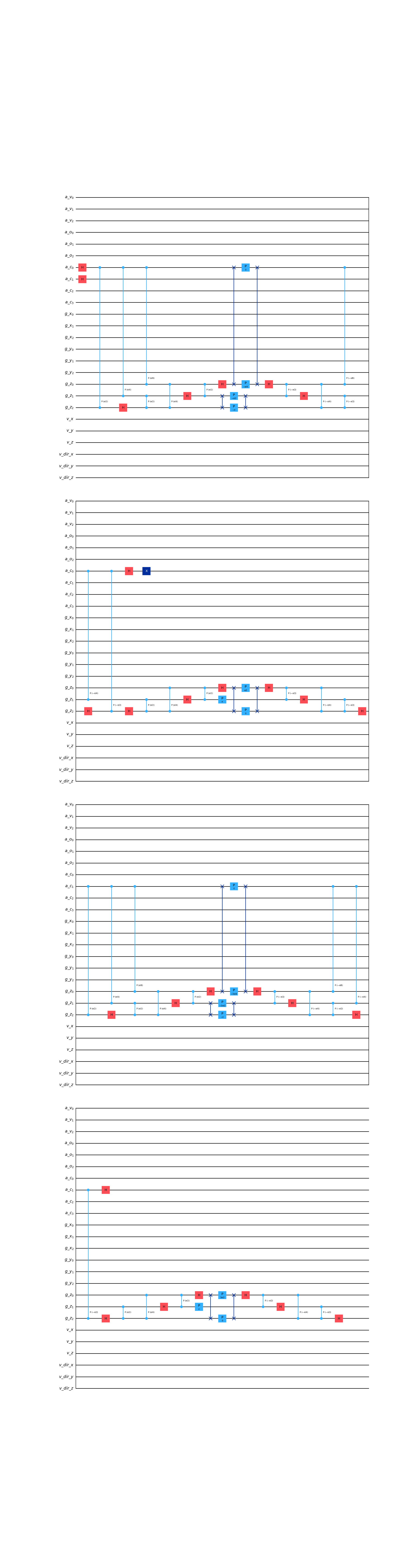
from qlbm.components.ms import BounceBackWallComparator
from qlbm.lattice import MSLattice

# Build an example lattice
lattice = MSLattice(
    {
        "lattice": {"dim": {"x": 8, "y": 8}, "velocities": {"x": 4, "y": 4}},
        "geometry": [{"shape":"cuboid", "x": [5, 6], "y": [1, 2], "boundary": "bounceback"}],
    }
)

# Comparing on the indices of the inside x-wall on the lower-bound of the obstacle
BounceBackWallComparator(
    lattice=lattice, wall=lattice.shape_list[0].walls_inside[0][0]
).draw("mpl")
(
Source code,png,hires.png,pdf)
- Parameters:
lattice (MSLattice)
wall (ReflectionWall)
logger (Logger)
- class qlbm.components.ms.specular_reflection.SpecularWallComparator(lattice, wall, logger=<Logger qlbm (WARNING)>)[source]#
A primitive used in the collisionless
SpecularReflectionOperatorthat implements the comparator for the specular reflection boundary conditions around the wall as described Schalkers and Möller [10].The comparator sets the d ancilla qubits to \(\ket{1}\) for the components of the quantum state whose grid qubits fall within the range spanned by the wall.
Attribute
Summary
latticeThe
AmplitudeLatticebased on which the properties of the operator are inferred.wallThe
ReflectionWallencoding the range spanned by the wall.loggerThe performance logger, by default
getLogger("qlbm").Example usage:
from qlbm.components.ms import SpecularWallComparator
from qlbm.lattice import MSLattice

# Build an example lattice
lattice = MSLattice(
    {
        "lattice": {"dim": {"x": 8, "y": 8}, "velocities": {"x": 4, "y": 4}},
        "geometry": [{"shape":"cuboid", "x": [5, 6], "y": [1, 2], "boundary": "specular"}],
    }
)

# Comparing on the indices of the inside x-wall on the lower-bound of the obstacle
SpecularWallComparator(
    lattice=lattice, wall=lattice.shape_list[0].walls_inside[0][0]
).draw("mpl")
(
Source code,png,hires.png,pdf)
- Parameters:
lattice (AmplitudeLattice)
wall (ReflectionWall)
logger (Logger)
- class qlbm.components.ms.primitives.EdgeComparator(lattice, edge, logger=<Logger qlbm (WARNING)>)[source]#
A primitive used in the 3D collisionless
SpecularReflectionOperatorandBounceBackReflectionOperatordescribed in Schalkers and Möller [10].Attribute
Summary
latticeThe
MSLatticebased on which the properties of the operator are inferred.loggerThe performance logger, by default
getLogger("qlbm").edgeThe coordinates of the edge within the grid.
Example usage:
from qlbm.components.ms import EdgeComparator
from qlbm.lattice import MSLattice

# Build an example lattice
lattice = MSLattice(
    {
        "lattice": {
            "dim": {"x": 8, "y": 8, "z": 8},
            "velocities": {"x": 4, "y": 4, "z": 4},
        },
        "geometry": [{"shape":"cuboid", "x": [2, 5], "y": [2, 5], "z": [2, 5], "boundary": "specular"}],
    }
)

# Draw the edge comparator circuit for one specific corner edge
EdgeComparator(lattice, lattice.shape_list[0].corner_edges_3d[0]).draw("mpl")
(
Source code,png,hires.png,pdf)
- Parameters:
lattice (MSLattice)
edge (ReflectionResetEdge)
logger (Logger)
Note
The amplitude-based QLBM supports two kinds of reflection operators: segment-wise (or standard) and zone-agnostic. The two methods are physically equivalent, but their implementation differs algorithmically. For multi-geometry cases, only the segment-wise implementation is currently supported.
- class qlbm.components.ab.reflection.ABReflectionOperator(lattice, shapes=None, logger=<Logger qlbm (WARNING)>)[source]#
Implements reflection boundary conditions in the amplitude-based encoding of
ABQLBMfor \(D_dQ_q\) discretizations.This is the top-level entrypoint that delegates to
ABBounceBackReflectionOperatorandABSpecularReflectionOperatorbased on the boundary condition types present in the geometry.Example usage:
from qlbm.components.ab import ABReflectionOperator
from qlbm.lattice import ABLattice

lattice = ABLattice(
    {
        "lattice": {"dim": {"x": 4, "y": 4}, "velocities": "d2q9"},
        "geometry": [
            {
                "shape": "cuboid",
                "x": [1, 3],
                "y": [1, 3],
                "boundary": "bounceback",
            }
        ],
    }
)

ABReflectionOperator(lattice).draw("mpl")
(
Source code,png,hires.png,pdf)
- Parameters:
lattice (AmplitudeLattice)
shapes (Dict[str, List[Shape]] | None)
logger (Logger)
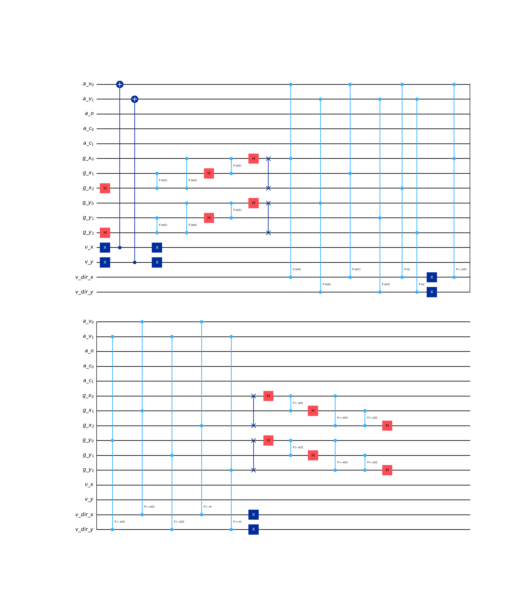
- class qlbm.components.ab.reflection.ABBounceBackReflectionOperator(lattice, blocks, control_on_marker_state=False, logger=<Logger qlbm (WARNING)>)[source]#
Implements bounce-back reflection in the amplitude-based encoding of
ABQLBMfor \(D_2Q_9\).Bounce-back reflection reverses all velocity components of particles that have entered the obstacle walls. The algorithm proceeds as:
Mark inner walls – Set the obstacle ancilla for gridpoints inside each wall segment.
Mark inner corners – Set the obstacle ancilla for the inner corner gridpoints.
Permute and stream – Apply the bounce-back velocity permutation (full reversal) and stream, both controlled on the obstacle ancilla.
Reset outer walls – Reset the obstacle ancilla using the outside wall comparators.
Corner corrections – Fix near-corner and outside-corner ancilla residuals.
- Parameters:
lattice (AmplitudeLattice)
blocks (List[Shape])
control_on_marker_state (bool)
logger (Logger)
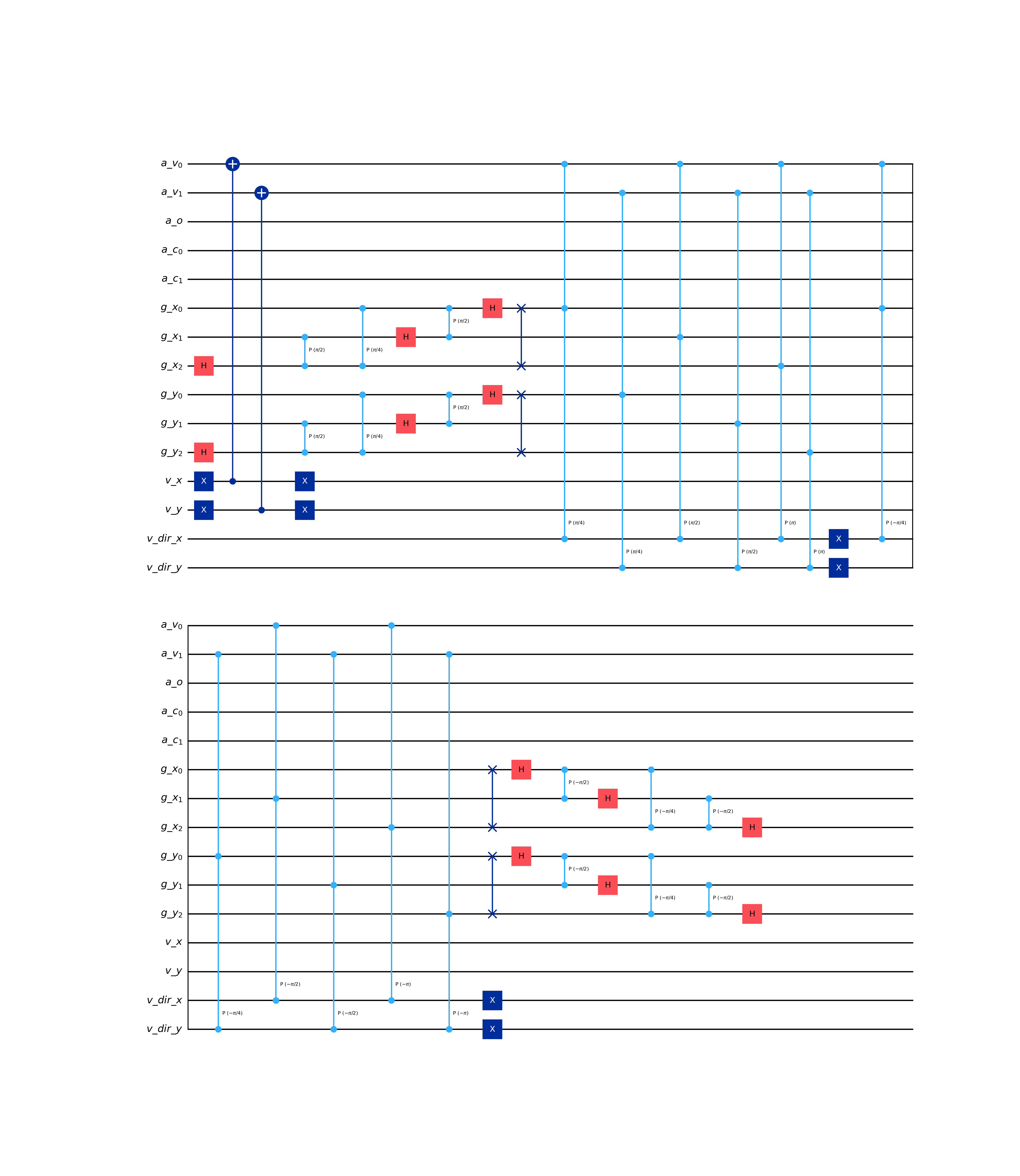
- class qlbm.components.ab.reflection.ABSpecularReflectionOperator(lattice, blocks, control_on_marker_state=False, logger=<Logger qlbm (WARNING)>)[source]#
Implements specular reflection in the amplitude-based encoding of
ABQLBMfor \(D_2Q_9\).This operator uses per-dimension obstacle ancillae (
a_x,a_y) to track which wall a particle has entered through. The algorithm proceeds in five phases:Mark inner walls – For each dimension, set the per-dimension obstacle ancilla for all gridpoints lying inside the walls of each block.
Specular permutations – Apply per-dimension velocity permutations controlled on the corresponding obstacle ancilla.
Dimension-selective stream – For each dimension d, stream the grid qubits of d controlled on
ancilla[d]. This ensures a particle reflected off an x-wall only moves in x, while a corner particle (both ancillae set) moves in both.Reset outer walls – For each dimension, reset the per-dimension obstacle ancilla using the outside wall comparators.
Corner corrections – Fix near-corner and outside-corner ancilla residuals caused by the wall-based reset overshoot and by cardinal velocities at inner corners.
- class qlbm.components.ab.reflection.ABZoneAgnosticReflectionOperator(lattice, shapes=None, logger=<Logger qlbm (WARNING)>)[source]#
Implements bounceback reflection in the amplitude-based encoding of
ABQLBMfor \(D_dQ_q\) discretizations.Uses a zone-agnostic approach that relies on the existence of an oracle that marks the basis states belonging to the inside of the solid geometry. For more details on the oracle, see
ABZoneAgnosticReflectionOracle.Example usage:
from qlbm.components.ab import ABZoneAgnosticReflectionOperator
from qlbm.lattice import ABLattice

lattice = ABLattice(
    {
        "lattice": {"dim": {"x": 4, "y": 4}, "velocities": "d2q9"},
        "geometry": [
            {
                "shape": "cuboid",
                "x": [1, 3],
                "y": [1, 3],
                "boundary": "bounceback",
            }
        ],
    }
)

ABZoneAgnosticReflectionOperator(lattice).draw("mpl")
(
Source code,png,hires.png,pdf)
- class qlbm.components.ab.reflection.ABZoneAgnosticReflectionOracle(lattice, shape, control_on_marker_state=False, additional_control_qubits=[], target_obstacle_index=0, logger=<Logger qlbm (WARNING)>)[source]#
Implementation of the oracle required for
ABZoneAgnosticReflectionOperator.An oracle is an operator \(U_{\Omega}\) for an obstacle’s region \(\Omega\) such that, in the amplitude-based encoding, \(U_\Omega\ket{x}\ket{v}\ket{0}_\mathbb{o} = \ket{x}\ket{v}\ket{x \in \Omega}_\mathbb{o}\). Intuitively, the operator flips the object ancilla qubit if and only if the position \(x\) falls within the bounds of the object.
Currently, the only available implementation is for 2D axis-aligned
BlockandYMonomialobjects.Important
The
YMonomialimplementation is a work in progress. At present, only the \(x^2\) monomial case is supported, and only when the monomial result register width matches the \(y\) grid register width.This is an improvement in asymptotic and practical complexity compared to the methods described in [10]. This operation relies on basic arithmetic through the
ParameterizedDraperAdderclass and comparison operation through theComparatorcircuits.When
control_on_marker_stateisTrue, the oracle additionally conditions the obstacle ancilla flip on the marker register being in the all-ones state. This is used for parallel boundary conditions where multiple geometries are simulated on the same lattice, each identified by a marker state. Only the central MCX gate (for cuboids) is controlled on the marker, since the surrounding adder and comparator operations are self-inverse and their net effect on the grid register is zero.Important
Marker-controlled oracles for
YMonomialshapes are not yet supported. Passingcontrol_on_marker_state=Truewith aYMonomialshape will raise aCircuitException.Example usage for a cuboid
Block:from qlbm.components.ab.reflection import ABZoneAgnosticReflectionOracle from qlbm.lattice import ABLattice lattice = ABLattice( { "lattice": {"dim": {"x": 4, "y": 16}, "velocities": "d2q9"}, "geometry": [ { "shape": "cuboid", "x": [1, 3], "y": [1, 3], "boundary": "bounceback", } ], } ) ABZoneAgnosticReflectionOracle(lattice, shape=lattice.shapes["bounceback"][0]).draw("mpl")
(
Source code,png,hires.png,pdf)
And for a
YMonomial:from qlbm.components.ab.reflection import ABZoneAgnosticReflectionOracle from qlbm.lattice import ABLattice lattice = ABLattice( { "lattice": {"dim": {"x": 4, "y": 16}, "velocities": "d2q9"}, "geometry": [ { "shape": "ymonomial", "exponent": 2, "comparator": "<", "boundary": "bounceback", } ], } ) ABZoneAgnosticReflectionOracle(lattice, shape=lattice.shapes["bounceback"][0]).draw("mpl")
(
Source code,png,hires.png,pdf)
Measurement#
- class qlbm.components.ms.primitives.GridMeasurement(lattice, logger=<Logger qlbm (WARNING)>)[source]#
A primitive that implements a measurement operation on the grid qubits.
Used at the end of the time step circuit to extract information from the quantum state.
Attribute
Summary
latticeThe
MSLatticebased on which the properties of the operator are inferred.loggerThe performance logger, by default
getLogger("qlbm").Example usage:
from qlbm.components.ms import GridMeasurement
from qlbm.lattice import MSLattice

# Build an example lattice
lattice = MSLattice({
    "lattice": {
        "dim": {
                "x": 8,
                "y": 8
            },
            "velocities": {
                "x": 4,
                "y": 4
        }
    },
    "geometry": [
        {
            "shape": "cuboid",
            "x": [5, 6],
            "y": [1, 2],
            "boundary": "specular"
        }
    ]
})

# Draw the measurement circuit
GridMeasurement(lattice).draw("mpl")
(
Source code,png,hires.png,pdf)
- Parameters:
lattice (MSLattice)
logger (Logger)
- class qlbm.components.ab.measurement.ABGridMeasurement(lattice, measure_velocity_qubits=False, logger=<Logger qlbm (WARNING)>)[source]#
Grid measurement for the
ABQLBMalgorithm.Example usage:
from qlbm.components.ab import ABGridMeasurement
from qlbm.lattice import ABLattice

lattice = ABLattice(
    {
        "lattice": {"dim": {"x": 32, "y": 8}, "velocities": "d2q9"},
        "geometry": [],
    }
)

ABGridMeasurement(lattice).draw("mpl")
(
Source code,png,hires.png,pdf)
- Parameters:
lattice (ABLattice)
measure_velocity_qubits (bool)
logger (Logger)