QLGA Circuits#
This page contains documentation about the quantum circuits that make up the
Lattice Gas Automata (LGA) algorithms of qlbm.
This includes two aglorithms:
At its core, the Space-Time QLBM uses an extended computational basis state encoding that that circumvents the non-locality of the streaming step by including additional information from neighboring grid points. This happens in several distinct steps: The LQGLA encodes a lattice of \(N_g\) gridpoints with \(q\) discrete velocities each into \(N_g \cdot q\) qubits. LQLGA can be seen as the “limit” of the extended computational basis state encoding that is the Space-Time encoding. For both algorithms, time-evolution of the system consists of the following steps:
Initial Conditions prepare the starting state of the flow field.
Streaming move particles across gridpoints according to the velocity discretization.
Reflection circuits apply boundary conditions that affect particles that come in contact with solid obstacles. Reflection places those particles back in the appropriate position of the fluid domain.
Collision operators create superposed local configurations of velocity profiles.
Measurement operations extract information out of the quantum state, which can later be post-processed classically.
This page documents the individual components that make up the CQLBM algorithm. Subsections follow a top-down approach, where end-to-end operators are introduced first, before being broken down into their constituent parts.
Warning
STQLBM and LQLGA are a based on typical \(D_dQ_q\) discretizations.
The current implementation only supports \(D_1Q_2\), \(D_1Q_3\), and \(D_2Q_4\) for one time step
with inexact restarts through qlbm‘s reinitialization mechanism.
LQLGA only supports \(D_1Q_3\).
Note
Need to work with a different discretization or want to work together? Reach out at qcfd-ewi@tudelft.nl.
End-to-end algorithms#
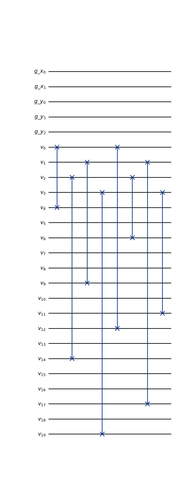
- class qlbm.components.spacetime.spacetime.SpaceTimeQLBM(lattice, filter_inside_blocks=True, logger=<Logger qlbm (WARNING)>)[source]#
The end-to-end algorithm of the Space-Time Quantum Lattice Boltzmann Algorithm described in [12].
This implementation currently only supports 1 time step on the \(D_2Q_4\) lattice discretization. Additional steps are possible by means of reinitialization.
The algorithm is composed of two main steps, the implementation of which (in general) varies per individual time step:
Streaming performed by the
SpaceTimeStreamingOperatormoves the particles on the grid by means of swap gates over velocity qubits.Collision performed by the
GenericSpaceTimeCollisionOperatordoes not move particles on the grid, but locally alters the velocity qubits at each grid point, if applicable.
Attribute
Summary
latticeThe
SpaceTimeLatticebased on which the properties of the operator are inferred.loggerThe performance logger, by default
getLogger("qlbm").Example usage:
from qlbm.components.spacetime import SpaceTimeQLBM
from qlbm.lattice import SpaceTimeLattice

# Build an example lattice
lattice = SpaceTimeLattice(
    num_timesteps=1,
    lattice_data={
        "lattice": {"dim": {"x": 4, "y": 8}, "velocities": "D2Q4"},
        "geometry": [],
    },
)

# Draw the end-to-end algorithm for 1 time step
SpaceTimeQLBM(lattice=lattice).draw("mpl")
(
Source code,png,hires.png,pdf)
- Parameters:
lattice (SpaceTimeLattice)
filter_inside_blocks (bool)
logger (Logger)
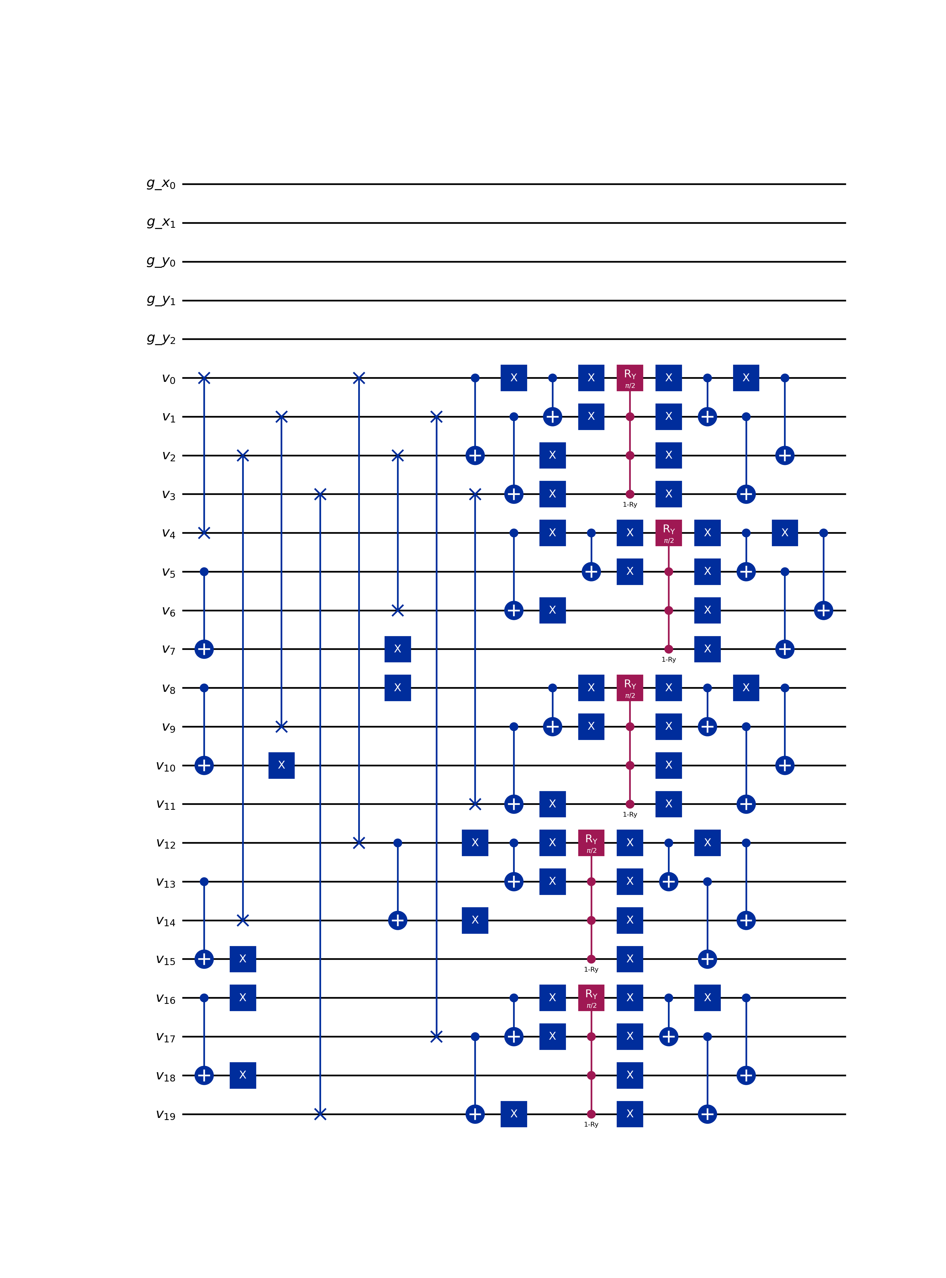
- class qlbm.components.LQLGA(lattice, logger=<Logger qlbm (WARNING)>)[source]#
Implementation of the Linear Quantum Lattice Gas Algorithm (LQLGA).
For a lattice with \(N_g\) gridpoints and \(q\) discrete velocities, LQLGA requires exactly \(N_g \cdot q\) qubits.
That is exactly equal to the number of classical bits required for one deterministic run of the classical LGA algorithm.
More information about this algorithm can be found in Love [9], Kocherla et al. [8], and Georgescu et al. [6].
Example usage:
from qlbm.components.lqlga import LQLGA
from qlbm.lattice import LQLGALattice

lattice = LQLGALattice(
    {
        "lattice": {
            "dim": {"x": 7},
            "velocities": "D1Q3",
        },
        "geometry": [{"shape": "cuboid", "x": [3, 5], "boundary": "bounceback"}],
    },
)

LQLGA(lattice=lattice).draw("mpl")
(
Source code,png,hires.png,pdf)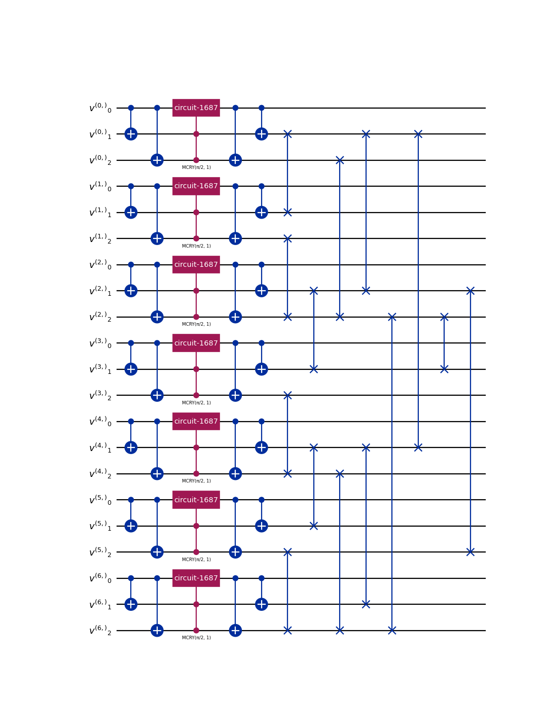
- Parameters:
lattice (LQLGALattice)
logger (Logger)
Initial Conditions#
- class qlbm.components.spacetime.initial.PointWiseSpaceTimeInitialConditions(lattice, grid_data=[((2, 5), (True, True, True, True)), ((3, 4), (False, True, False, True))], filter_inside_blocks=True, logger=<Logger qlbm (WARNING)>)[source]#
Prepares the initial state for the
SpaceTimeQLBM.Initial conditions are supplied in a
List[Tuple[Tuple[int, int], Tuple[bool, bool, bool, bool]]]containing, for each population to be initialized, two nested tuples.The first tuple position of the population(s) on the grid (i.e.,
(2, 5)). The second tuple contains velocity of the population(s) at that location. Since the maximum number of velocities is pre-determined and the computational basis state encoding favors boolean logic, the input is provided as a tuple ofbooleans. That is,(True, True, False, False)would mean there are two populations at the same gridpoint, with velocities \(q_0\) and \(q_1\) according to the \(D_2Q_4\) discretization. Together, thegrid_dataargument of the constructor can be supplied as, for instance,[((3, 7), (False, True, False, True))].The initialization follows the following steps:
- For each (position, velocity) pair:
Set the gird qubits encoding the position to \(\ket{1}^{\otimes n_g}\) using \(X\) gates;
Set each of the toggled velocities to \(\ket{1}\) by means of \(MCX\) gates, controlled on the qubits set in the previous step;
Undo the operation of step 1 (i.e., repeat the \(X\) gates);
Repeat steps 1-3 for all neighboring velocity qubits, adjusting for grid position and relative velocity index.
Attribute
Summary
grid_dataThe information encoding the particle probability distribution, formatted as (position, velocity) tuples.
latticeThe
SpaceTimeLatticebased on which the properties of the operator are inferred.loggerThe performance logger, by default
getLogger("qlbm").Example usage:
from qlbm.components.spacetime.initial import PointWiseSpaceTimeInitialConditions
from qlbm.lattice import SpaceTimeLattice

# Build an example lattice
lattice = SpaceTimeLattice(
    num_timesteps=1,
    lattice_data={
        "lattice": {"dim": {"x": 4, "y": 8}, "velocities": "D2Q4"},
        "geometry": [],
    },
)

# Draw the initial conditions for two particles at (3, 7), traveling in the +y and -y directions
PointWiseSpaceTimeInitialConditions(lattice=lattice, grid_data=[((3, 7), (False, True, False, True))]).draw("mpl")
(
Source code,png,hires.png,pdf)
- Parameters:
lattice (SpaceTimeLattice)
grid_data (List[Tuple[Tuple[int, ...], Tuple[bool, ...]]])
filter_inside_blocks (bool)
logger (Logger)
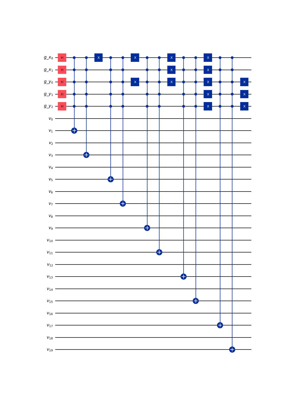
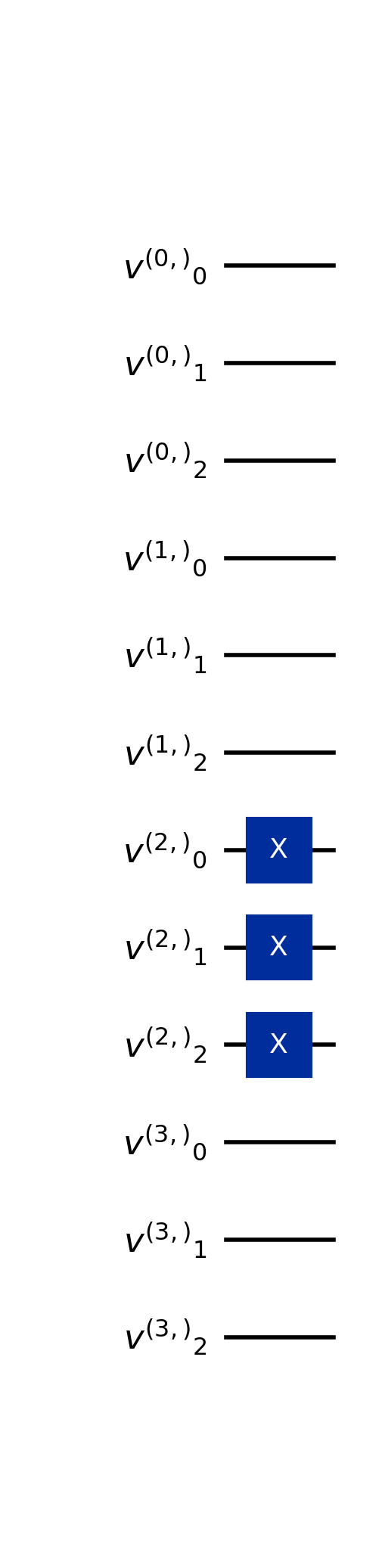
- class qlbm.components.LQGLAInitialConditions(lattice, grid_data, logger=<Logger qlbm (WARNING)>)[source]#
Primitive for setting initial conditions in the
LQLGAalgorithm.This operator allows the construction of arbitrary deterministic initial conditions for the LQLGA algorithm. The number of gates required by this operator is equal to the number of enabled velocity qubits across all grid points. The depth of the circuit is 1, as all gates are applied in parallel at each grid point.
Example usage:
from qlbm.lattice import LQLGALattice
from qlbm.components.lqlga import LQGLAInitialConditions

lattice = LQLGALattice(
    {
        "lattice": {
            "dim": {"x": 4},
            "velocities": "D1Q3",
        },
        "geometry": [],
    },
)
initial_conditions = LQGLAInitialConditions(lattice, [(tuple([2]), (True, True, True))])
initial_conditions.draw("mpl")
(
Source code,png,hires.png,pdf)
- Parameters:
lattice (LQLGALattice)
grid_data (List[Tuple[Tuple[int, ...], Tuple[bool, ...]]])
logger (Logger)
Streaming#
- class qlbm.components.spacetime.streaming.SpaceTimeStreamingOperator(lattice, timestep, logger=<Logger qlbm (WARNING)>)[source]#
An operator that performs streaming as a series of \(SWAP\) gates as part of the
SpaceTimeQLBMalgorithm.The velocities corresponding to neighboring gridpoints are streamed “into” the gridpoint affected relative to the
timestep. The register setup of theSpaceTimeLatticeis such that following each time step, an additional “layer” neighboring velocity qubits can be discarded, since the information they encode can never reach the relative origin in the remaining number of time steps. As such, the complexity of the streaming operator decreases with the number of steps (still) to be simulated. For an in-depth mathematical explanation of the procedure, consult pages 15-18 of Schalkers and Möller [12].Attribute
Summary
latticeThe
SpaceTimeLatticebased on which the properties of the operator are inferred.timestepThe time step for which to perform streaming.
loggerThe performance logger, by default
getLogger("qlbm").Example usage:
from qlbm.components.spacetime import SpaceTimeStreamingOperator
from qlbm.lattice import SpaceTimeLattice

# Build an example lattice
lattice = SpaceTimeLattice(
    num_timesteps=1,
    lattice_data={
        "lattice": {"dim": {"x": 4, "y": 8}, "velocities": "D2Q4"},
        "geometry": [],
    },
)

# Draw the streaming operator for 1 time step
SpaceTimeStreamingOperator(lattice=lattice, timestep=1).draw("mpl")
(
Source code,png,hires.png,pdf)
- Parameters:
lattice (SpaceTimeLattice)
timestep (int)
logger (Logger)
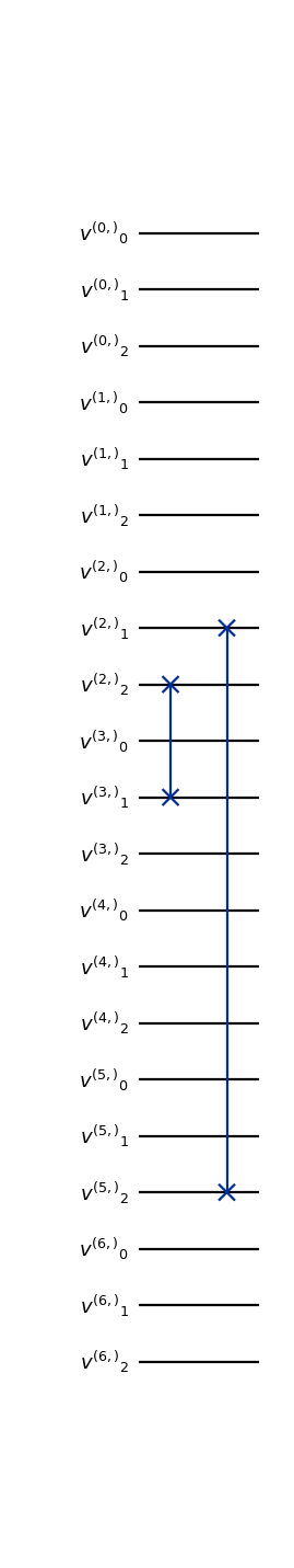
- class qlbm.components.LQLGAStreamingOperator(lattice, logger=<Logger qlbm (WARNING)>)[source]#
Streaming operator for the
LQLGAalgorithm.Streaming is implemented by a series of swap gates as described in [12]. The number of gates scales linearly with size of the grid, while the depth scales logarithmically.
Example usage:
from qlbm.components.lqlga import LQLGAStreamingOperator
from qlbm.lattice import LQLGALattice

lattice = LQLGALattice(
    {
        "lattice": {
            "dim": {"x": 4},
            "velocities": "D1Q3",
        },
        "geometry": [],
    },
)
streaming_operator = LQLGAStreamingOperator(lattice)
streaming_operator.draw("mpl")
(
Source code,png,hires.png,pdf)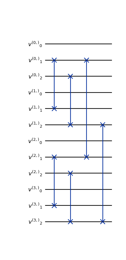
- Parameters:
lattice (LQLGALattice)
logger (Logger)
Reflection#
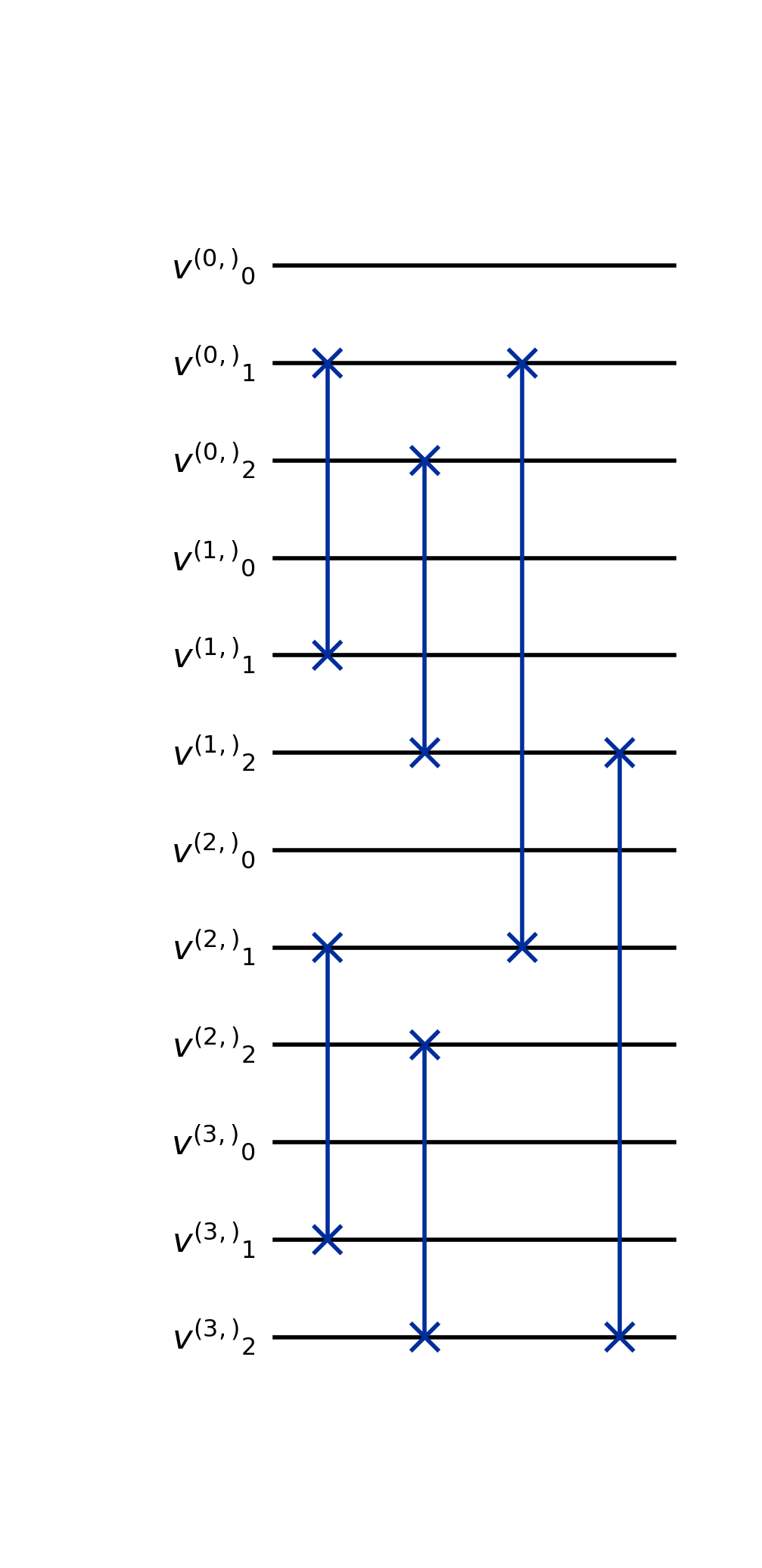
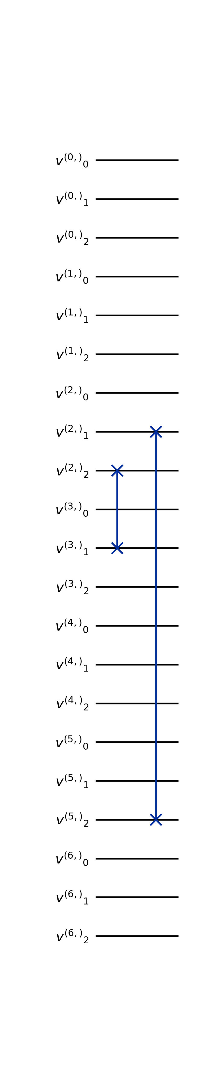
- class qlbm.components.LQLGAReflectionOperator(lattice, shapes, logger=<Logger qlbm (WARNING)>)[source]#
Operator implementing reflection in the
LQLGAalgorithm.Reflections in this algorithm can be entirely implemented by swap gates. The number of gates scales with the number of gridpoints of the solid geometry. The depth of the operator is 1.
Attribute
Summary
latticeThe lattice the operator acts on.
shapesA list of boundary-conditioned shapes.
loggerThe performance logger, by default
getLogger("qlbm").Example usage:
from qlbm.components.lqlga import LQLGAReflectionOperator
from qlbm.lattice import LQLGALattice

lattice = LQLGALattice(
    {
        "lattice": {
            "dim": {"x": 7},
            "velocities": "D1Q3",
        },
        "geometry": [{"shape": "cuboid", "x": [3, 5], "boundary": "bounceback"}],
    },
)
reflection_operator = LQLGAReflectionOperator(
    lattice, shapes=lattice.shapes["bounceback"]
)
reflection_operator.draw("mpl")
(
Source code,png,hires.png,pdf)
- Parameters:
lattice (LQLGALattice)
shapes (List[LQLGAShape])
logger (Logger)
Collision#
The collision module contains collision operators and adjacent logic classes. The former implements the circuits that perform collision in computational basis state encodings, while the latter contains useful abstractions that circuits build on top of. Collision in LGA algorithms is based on the concept of equivalence classes described in Section 4 of [6], and follows a permute-redistribute-unpermute (PRP) approach. All components of this module may be used for different variations of the Computational Basis State Encoding (CBSE) of the velocity register. The components of this module consist of:
- class qlbm.components.spacetime.collision.GenericSpaceTimeCollisionOperator(lattice, timestep, logger=<Logger qlbm (WARNING)>)[source]#
A generic space-time collision operator that can be used to apply any gate to the velocities of a grid location.
Attribute
Summary
latticeThe
SpaceTimeLatticebased on which the properties of the operator are inferred.gateThe gate to apply to the velocities.
loggerThe performance logger, by default
getLogger("qlbm").- Parameters:
lattice (SpaceTimeLattice)
timestep (int)
logger (Logger)
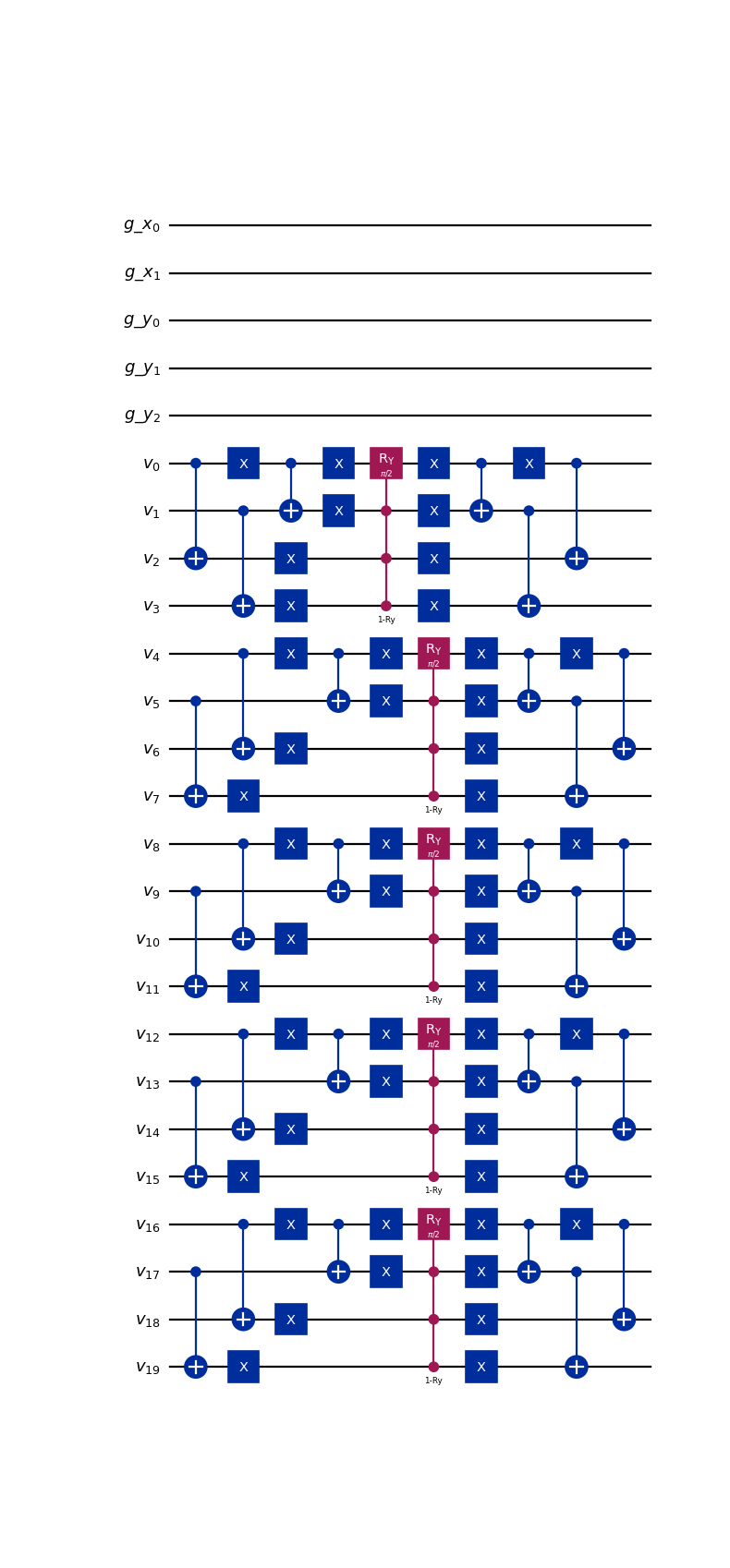
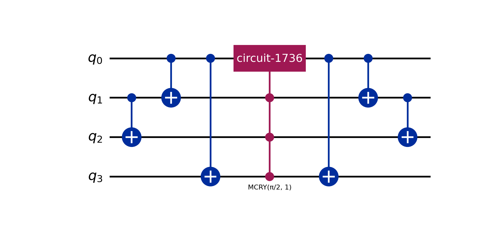
- class qlbm.components.spacetime.collision.SpaceTimeD2Q4CollisionOperator(lattice, timestep, gate_to_apply=Instruction(name='ry', num_qubits=1, num_clbits=0, params=[1.5707963267948966]), logger=<Logger qlbm (WARNING)>)[source]#
An operator that performs collision part of the
SpaceTimeQLBMalgorithm.Collision is a local operation that is performed simultaneously on all velocity qubits corresponding to a grid location. In practice, this means the same circuit is repeated across all “local” qubit register chunks. Collision can be understood as follows:
For each group of qubits, the states encoding velocities belonging to a particular equivalence class are first isolated with a series of \(X\) and \(CX\) gates. This leaves qubits not affected by the rotation in \(\ket{1}^{\otimes n_v-1}\) state.
A rotation gate is applied to the qubit(s) relevant to the equivalence class shift, controlled on the qubits set in the previous step.
The operation performed in Step 1 is undone.
The register setup of the
SpaceTimeLatticeis such that following each time step, an additional “layer” neighboring velocity qubits can be discarded, since the information they encode can never reach the relative origin in the remaining number of time steps. As such, the complexity of the collision operator decreases with the number of steps (still) to be simulated. For an in-depth mathematical explanation of the procedure, consult pages 11-15 of Schalkers and Möller [12].Attribute
Summary
latticeThe
SpaceTimeLatticebased on which the properties of the operator are inferred.timestepThe time step for which to perform streaming.
gate_to_applyThe gate to apply to the velocities matching equivalence classes. Defaults to \(R_y(\frac{\pi}{2})\).
loggerThe performance logger, by default
getLogger("qlbm").Example usage:
from qlbm.components.spacetime.collision.d2q4_old import SpaceTimeD2Q4CollisionOperator
from qlbm.lattice import SpaceTimeLattice

# Build an example lattice
lattice = SpaceTimeLattice(
    num_timesteps=1,
    lattice_data={
        "lattice": {"dim": {"x": 4, "y": 8}, "velocities": "D2Q4"},
        "geometry": [],
    },
)

# Draw the collision operator for 1 time step
SpaceTimeD2Q4CollisionOperator(lattice=lattice, timestep=1).draw("mpl")
(
Source code,png,hires.png,pdf)
- Parameters:
lattice (SpaceTimeLattice)
timestep (int)
gate_to_apply (Gate)
logger (Logger)
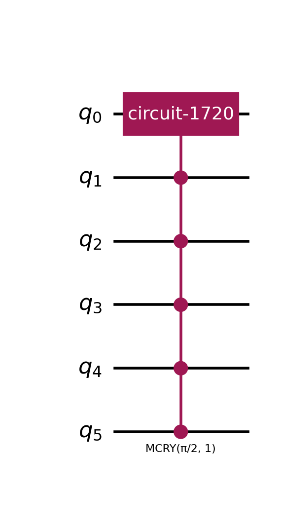
- class qlbm.components.GenericLQLGACollisionOperator(lattice, logger=<Logger qlbm (WARNING)>)[source]#
Equivalence class-based LGA collision operator for the
LQLGAalgorithm.This operator applies the
EQCCollisionOperatoroperator to all velocity qubits at each grid point.- Parameters:
lattice (LQLGALattice)
logger (Logger)
- class qlbm.components.common.EQCPermutation(equivalence_class, inverse=False, logger=<Logger qlbm (WARNING)>)[source]#
Applies a permutation to the velocity qubits of an equivalence Sclass in the CBSE encoding.
This is used as part of the PRP collision operator described in section 5 of [6]. Utilized in the
EQCCollisionOperator.Attribute Summary
equivalence_classThe equivalence class of the operator.
inverseWhether to apply the inverse permutation.
Example usage:
from qlbm.components.common import EQCPermutation
from qlbm.lattice import LatticeDiscretization
from qlbm.lattice.eqc import EquivalenceClassGenerator

# Generate some equivalence classes
eqcs = EquivalenceClassGenerator(
    LatticeDiscretization.D3Q6
).generate_equivalence_classes()

# Select one at random and draw its circuit
EQCPermutation(eqcs.pop(), inverse=False).circuit.draw("mpl")
(
Source code,png,hires.png,pdf)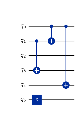
- Parameters:
equivalence_class (EquivalenceClass)
inverse (bool)
logger (Logger)
- class qlbm.components.common.EQCRedistribution(equivalence_class, decompose_block=True, logger=<Logger qlbm (WARNING)>)[source]#
Redistribution operator for equivalence classes in the CBSE encoding.
The operator is mathematically described in section 4 of [6]. Redistribution is applied before and after permutations, and consists of a controlled unitary operator composed of a discrete Fourier transform (DFT)-block matrix.
Attribute
Summary
equivalence_classThe equivalence class of the operator.
decompose_blockWhether to decompose the DFT block into a circuit.
Example usage:
from qlbm.components.common import EQCRedistribution
from qlbm.lattice import LatticeDiscretization
from qlbm.lattice.eqc import EquivalenceClassGenerator

# Generate some equivalence classes
eqcs = EquivalenceClassGenerator(
    LatticeDiscretization.D3Q6
).generate_equivalence_classes()

# Select one at random and draw its circuit in the schematic form
EQCRedistribution(eqcs.pop(), decompose_block=False).circuit.draw("mpl")
(
Source code,png,hires.png,pdf)
The decompose_block parameter can be set to
Trueto decompose the DFT block into a circuit:from qlbm.components.common import EQCRedistribution from qlbm.lattice import LatticeDiscretization from qlbm.lattice.eqc import EquivalenceClassGenerator # Generate some equivalence classes eqcs = EquivalenceClassGenerator( LatticeDiscretization.D3Q6 ).generate_equivalence_classes() # Select one at random and draw its decomposed circuit EQCRedistribution(eqcs.pop(), decompose_block=True).circuit.draw("mpl")
(
Source code,png,hires.png,pdf)
- Parameters:
equivalence_class (EquivalenceClass)
decompose_block (bool)
logger (Logger)
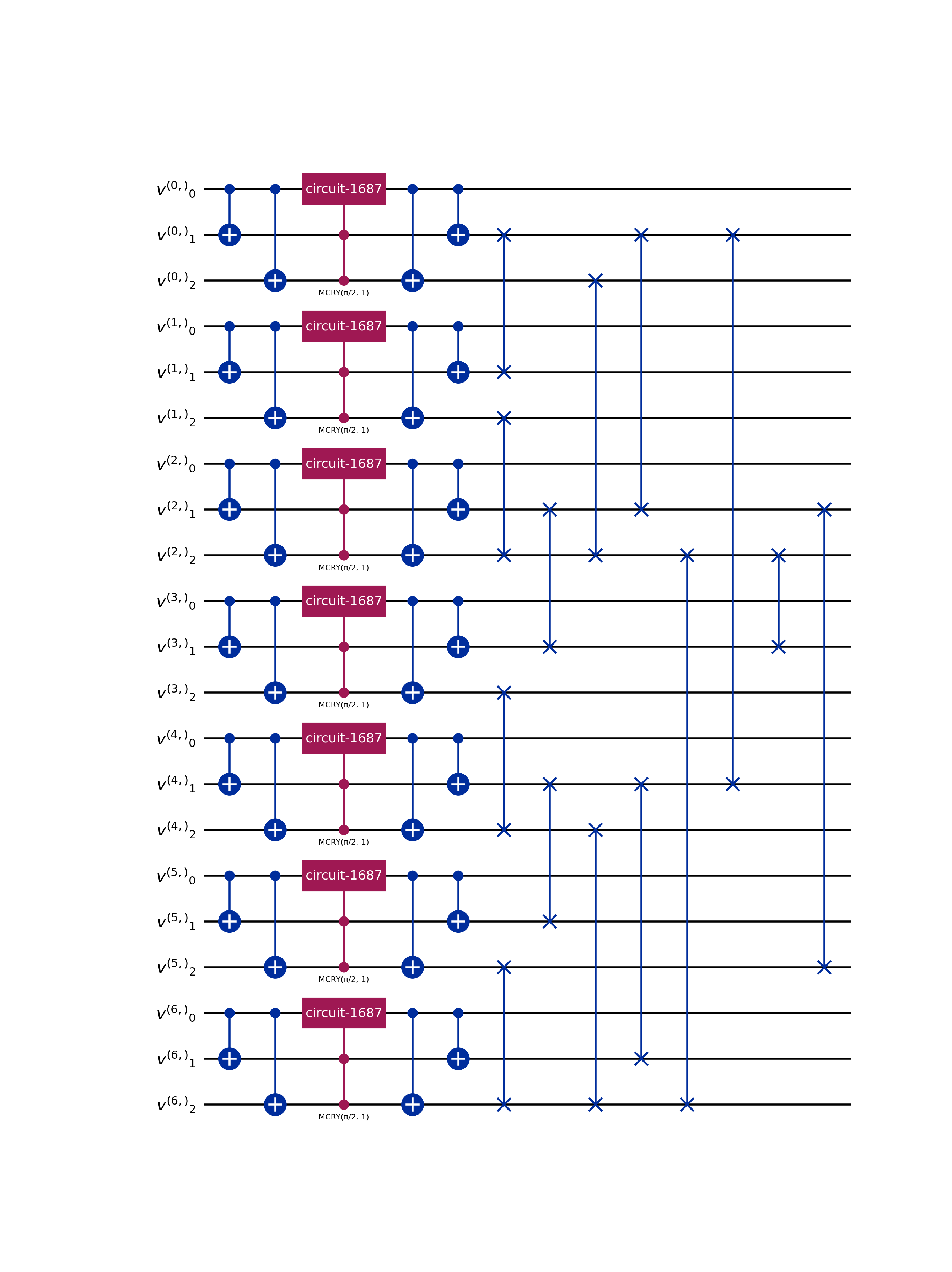
- class qlbm.components.common.EQCCollisionOperator(discretization)[source]#
Collision operator based on the equivalence class abstraction described in section 5 of [6].
Consists of a permutation, redistribution, and inverse permutation of the velocity qubits. This operator is designed to be applied to a single velocity register, which can be repeated depending on the encoding. Used in the
GenericSpaceTimeCollisionOperatorandGenericLQLGACollisionOperator.Attribute
Summary
discretizationThe discretization for which this collision operator is defined.
num_velocitiesThe number of velocities in the discretization.
Simple D2Q4 example usage:
from qlbm.components.common import EQCCollisionOperator
from qlbm.lattice import LatticeDiscretization

# Select a discretization and draw its circuit
EQCCollisionOperator(
    LatticeDiscretization.D2Q4
).draw("mpl")
(
Source code,png,hires.png,pdf)
More complex D3Q6 example usage:
from qlbm.components.common import EQCCollisionOperator
from qlbm.lattice import LatticeDiscretization

# Select a discretization and draw its circuit
EQCCollisionOperator(
    LatticeDiscretization.D3Q6
).draw("mpl")
(
Source code,png,hires.png,pdf)
- Parameters:
discretization (LatticeDiscretization)
- class qlbm.lattice.spacetime.properties_base.LatticeDiscretization(value, names=<not given>, *values, module=None, qualname=None, type=None, start=1, boundary=None)[source]#
The Lattice Boltzmann discretization used in the simulation.
The only supported discretizations currently are D1Q2 and D2Q4.
- class qlbm.lattice.spacetime.properties_base.LatticeDiscretizationProperties[source]#
Class containing properties of the lattice discretization in the \(D_dQ_q\) taxonomy.
Attributes# Attribute
Description
num_velocitiesThe number of velocities in the discretization. Stored as a
Dict[LatticeDiscretization, int].velocity_vectorsThe velocity profile each of the \(q\) velocity channels. Each vector is \(d\)-dimensional and each entry represents the velocity component of the channel in a particular dimension. Stored as a
Dict[LatticeDiscretization, numpy.ndarray].
- class qlbm.lattice.eqc.EquivalenceClass(discretization, velocity_configurations)[source]#
Class representing LGA equivalence classes.
In
qlbm, an equivalence class is a set of velocity configurations that share the same mass and momentum. For a more in depth explanation, consult Section 4 of [6].Constructor Attributes# Attribute
Description
discretizationThe
LatticeDiscretizationthat the equivalence class belongs to.velocity_configurationsThe
Set[Tuple[bool, ...]]that contains the velocity configurations of the equivalence class. Configurations are stored asq-tuples where an entry isTrueif the velocity channel is occupied andFalseotherwise.Class Attributes# Attribute
Description
massThe total mass of the equivalence class, which is the sum of all occupied velocity channels.
momentumThe total momentum of the equivalence class, which is the vector sum of all occupied velocity channels multiplid by their
LatticeDiscretizationPropertiesvelocity contribution.- Parameters:
discretization (LatticeDiscretization)
velocity_configurations (Set[Tuple[bool, ...]])
- class qlbm.lattice.eqc.EquivalenceClassGenerator(discretization)[source]#
A class that generates equivalence classes for a given lattice discretization.
Constructor Attributes# Attribute
Description
discretizationThe
LatticeDiscretizationthat the equivalence class belongs to.Example usage:
1from qlbm.lattice import LatticeDiscretization
2from qlbm.lattice.eqc import EquivalenceClassGenerator
3
4# Generate some equivalence classes
5eqcs = EquivalenceClassGenerator(
6    LatticeDiscretization.D3Q6
7).generate_equivalence_classes()
8
9print(eqcs.pop().get_bitstrings())
- Parameters:
discretization (LatticeDiscretization)
Measurement#
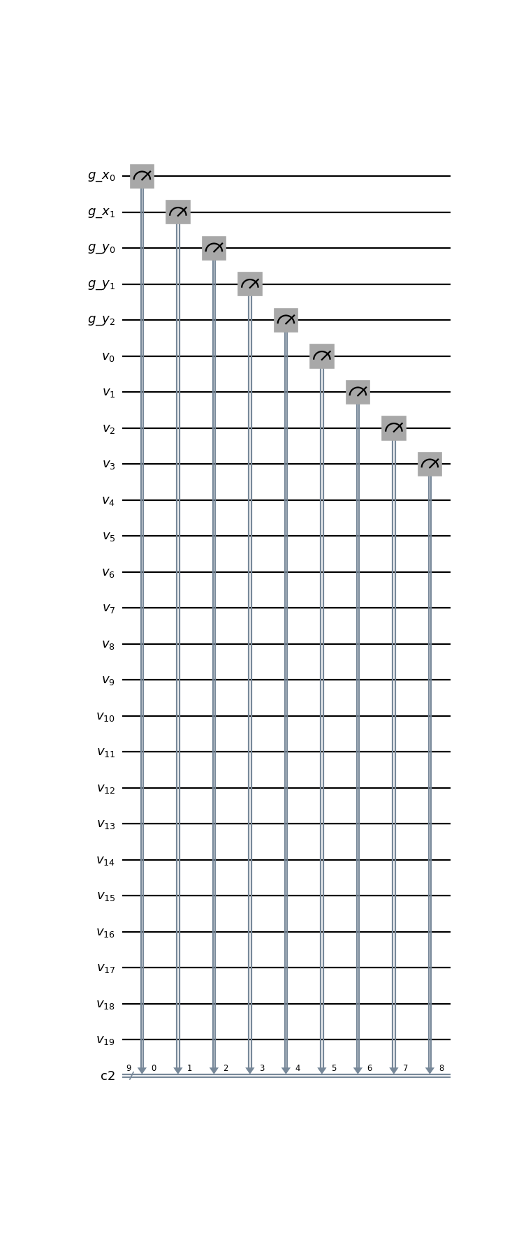
- class qlbm.components.spacetime.measurement.SpaceTimeGridVelocityMeasurement(lattice, logger=<Logger qlbm (WARNING)>)[source]#
A primitive that implements a measurement operation on the grid and the local velocity qubits.
Used at the end of the simulation to extract information from the quantum state. Together, the information from the local and grid qubits can be used for on-the-fly reinitialization.
Attribute
Summary
latticeThe
SpaceTimeLatticebased on which the properties of the operator are inferred.loggerThe performance logger, by default
getLogger("qlbm").Example usage:
from qlbm.components.spacetime import SpaceTimeGridVelocityMeasurement
from qlbm.lattice import SpaceTimeLattice

# Build an example lattice
lattice = SpaceTimeLattice(
    num_timesteps=1,
    lattice_data={
        "lattice": {"dim": {"x": 4, "y": 8}, "velocities": "D2Q4"},
        "geometry": [],
    },
)

# Draw the measurement circuit
SpaceTimeGridVelocityMeasurement(lattice=lattice).draw("mpl")
(
Source code,png,hires.png,pdf)
- Parameters:
lattice (SpaceTimeLattice)
logger (Logger)
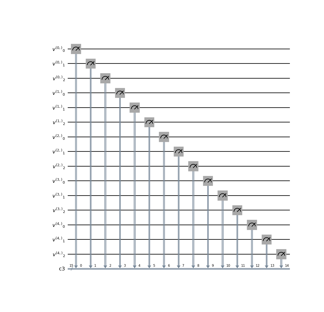
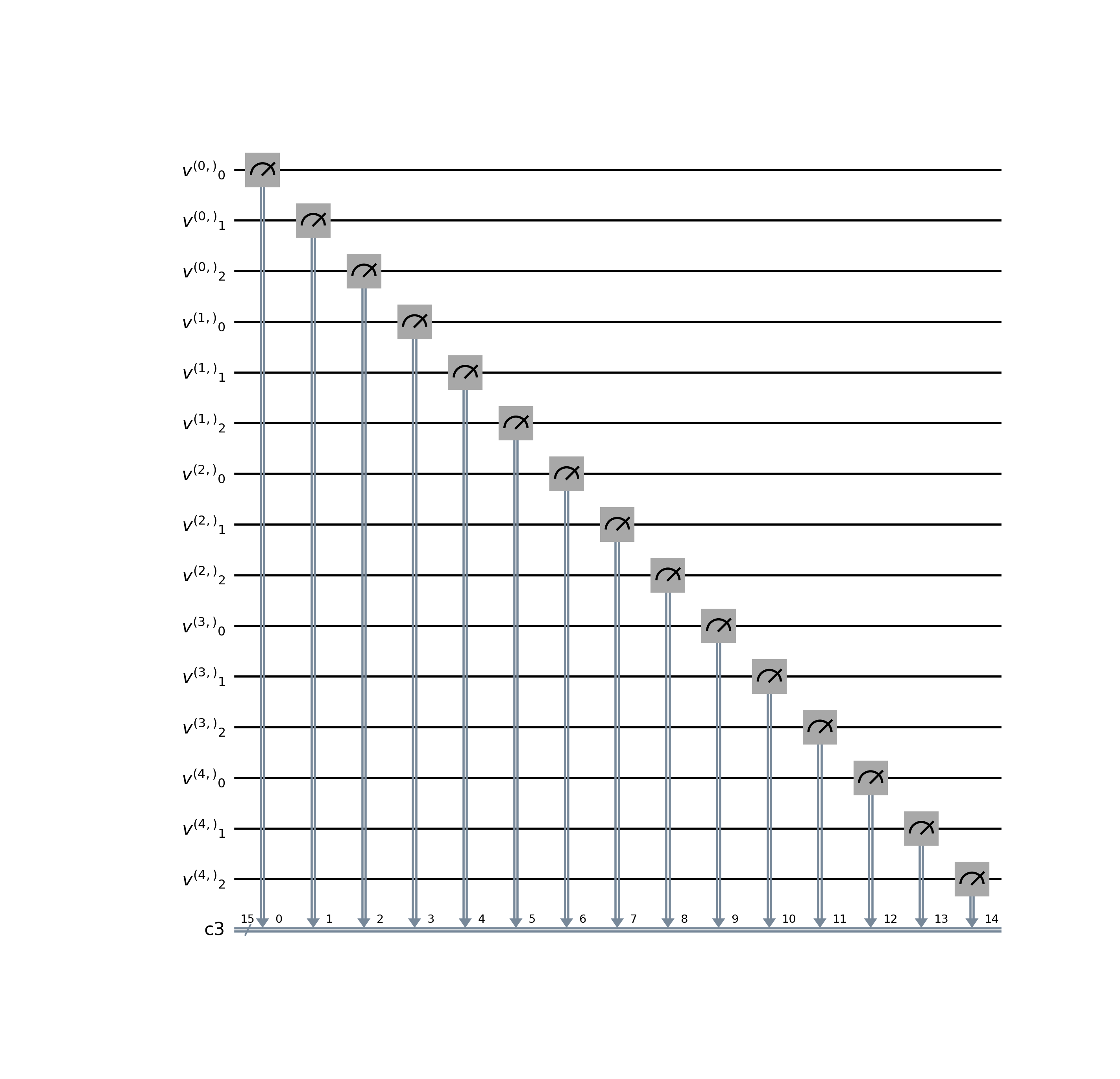
- class qlbm.components.LQLGAGridVelocityMeasurement(lattice, logger=<Logger qlbm (WARNING)>)[source]#
Measurement operator for the
LQLGAalgorithm.This operator measures the velocity qubits at each grid point in the LQLGA lattice.
Example usage:
from qlbm.components.lqlga import LQLGAGridVelocityMeasurement
from qlbm.lattice import LQLGALattice

lattice = LQLGALattice(
    {
        "lattice": {
            "dim": {"x": 5},
            "velocities": "D1Q3",
        },
        "geometry": [],
    },
)

LQLGAGridVelocityMeasurement(lattice=lattice).draw("mpl")
(
Source code,png,hires.png,pdf)
- Parameters:
lattice (LQLGALattice)
logger (Logger)