Collisionless Circuits#

This page contains documentation about the quantum circuits that make up the Collisionless Quantum Lattice Boltzmann Method (CQLBM) first described in [2] and later expanded in [3]. At its core, the CQLBM algorithm manipulates the particle probability distribution in an amplitude-based encoding of the quantum state. This happens in several distinct steps:

Initial conditions prepare the starting state of the probability distribution function.
Streaming circuits increment or decrement the position of particles in physical space through QFT-based streaming.
Reflection circuits apply boundary conditions that affect particles that come in contact with solid obstacles. Reflection places those particles back in the appropriate position of the fluid domain.
Measurement operations extract information out of the quantum state, which can later be post-processed classically.

This page documents the individual components that make up the CQLBM algorithm. Subsections follow a top-down approach, where end-to-end operators are introduced first, before being broken down into their constituent parts.

End-to-end algorithms#

class qlbm.components.collisionless.cqlbm.CQLBM(lattice, logger=<Logger qlbm (WARNING)>)[source]#

The end-to-end algorithm of the Collisionless Quantum Lattice Boltzmann Algorithm first introduced in Schalkers and Möller [2] and later extended in Schalkers and Möller [3].

This implementation supports 2D and 3D simulations with with cuboid objects with either bounce-back or specular reflection boundary conditions.

The algorithm is composed of three steps that are repeated according to a CFL counter:

Streaming performed by the CollisionlessStreamingOperator increments or decrements the positions of particles on the grid.
BounceBackReflectionOperator and SpecularReflectionOperator reflect the particles that come in contact with Block obstacles encoded in the CollisionlessLattice.
The StreamingAncillaPreparation resets the state of the ancilla qubits for the next CFL counter substep.

Attribute	Summary
`lattice`	The `CollisionlessLattice` based on which the properties of the operator are inferred.
`logger`	The performance logger, by default `getLogger("qlbm")`.

Parameters:

lattice (Lattice)
logger (Logger)

Streaming#

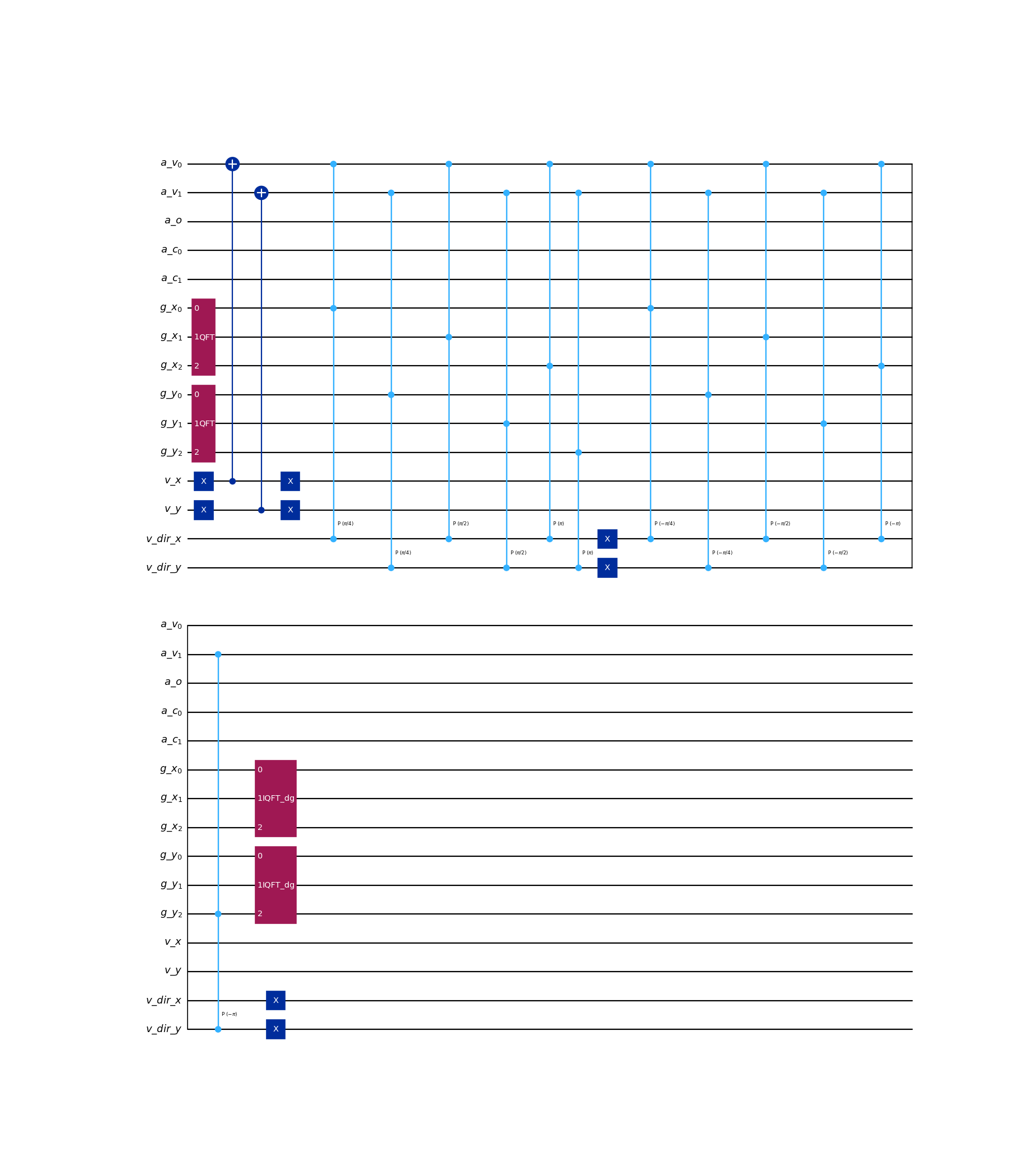
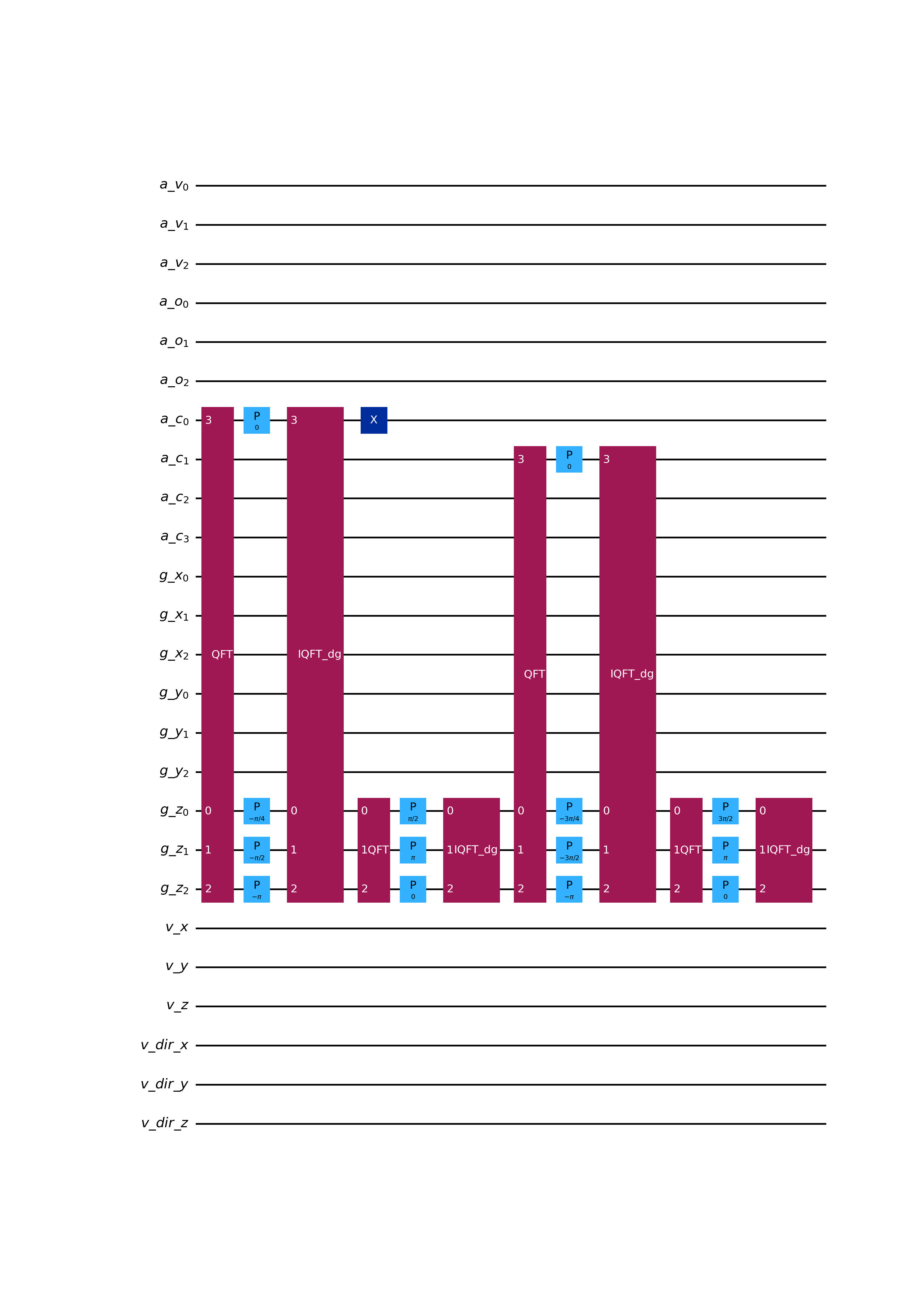
class qlbm.components.collisionless.streaming.CollisionlessStreamingOperator(lattice, velocities, logger=<Logger qlbm (WARNING)>)[source]#

An operator that performs streaming in Fourier space as part of the CQLBM algorithm.

Streaming is broken down into the following steps:

A StreamingAncillaPreparation object prepares the ancilla velocity qubits for CFL time step. This happens independently for all dimensions, and it is assumed the velocity discretization is uniform across dimensions.
A ControlledIncrementer performs incrementation or decrementation in the Fourier space, controlled on the ancilla qubits set in the previous steps.
For efficiency reasons, the velocity qubits set in step 1 are not reset, as they will be re-used in the subsequent reflection step. Another instance of the StreamingAncillaPreparation would be required to consistently end the step.

For an in-depth mathematical explanation of the procedure, consult Section 4 of Schalkers and Möller [2].

Attribute	Summary
`lattice`	The `CollisionlessLattice` based on which the properties of the operator are inferred.
`velocities`	A list of velocities to increment. This is computed according to CFL counter.
`logger`	The performance logger, by default `getLogger("qlbm")`.

Example usage:

from qlbm.components.collisionless import CollisionlessStreamingOperator
from qlbm.lattice import CollisionlessLattice

# Build an example lattice
lattice = CollisionlessLattice(
    {
        "lattice": {"dim": {"x": 8, "y": 8}, "velocities": {"x": 4, "y": 4}},
        "geometry": [],
    }
)

# Streaming the velocity with index 2
CollisionlessStreamingOperator(lattice=lattice, velocities=[2]).draw("mpl")

(Source code, png, hires.png, pdf)

Parameters:

lattice (CollisionlessLattice)
velocities (List[int])
logger (Logger)

class qlbm.components.collisionless.streaming.StreamingAncillaPreparation(lattice, velocities, dim, logger=<Logger qlbm (WARNING)>)[source]#

A primitive used in CollisionlessStreamingOperator that implements the preparatory step of streaming necessary for the CQLBM method.

This operator sets the ancilla qubits to \(\ket{1}\) for the velocities that will be streamed in the next CFL time step.

Attribute	Summary
`lattice`	The `CollisionlessLattice` based on which the properties of the operator are inferred.
`velocities`	The velocities that need to be streamed within the next time step.
`dim`	The dimension to which the velocities correspond.
`logger`	The performance logger, by default `getLogger("qlbm")`.

Example usage:

from qlbm.components.collisionless import StreamingAncillaPreparation
from qlbm.lattice import CollisionlessLattice

# Build an example lattice
lattice = CollisionlessLattice(
    {
        "lattice": {"dim": {"x": 8, "y": 8}, "velocities": {"x": 4, "y": 4}},
        "geometry": [],
    }
)

# Streaming velocities indexed 2 in the y (1) dimension
StreamingAncillaPreparation(lattice=lattice, velocities=[2], dim=1).draw("mpl")

(Source code, png, hires.png, pdf)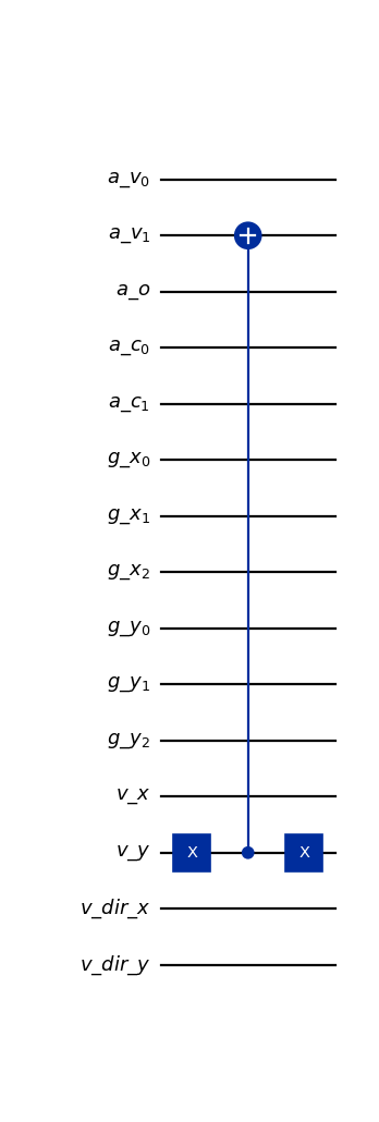

Parameters:

lattice (CollisionlessLattice)
velocities (List[int])
dim (int)
logger (Logger)

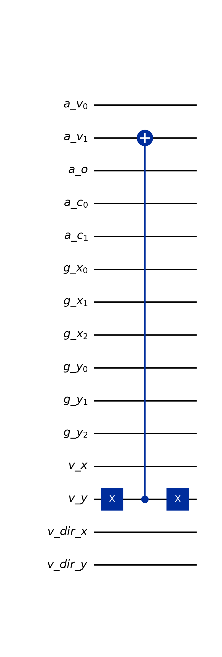
class qlbm.components.collisionless.streaming.ControlledIncrementer(lattice, reflection=None, logger=<Logger qlbm (WARNING)>)[source]#

A primitive used in CollisionlessStreamingOperator that implements the streaming operation on the states for which the ancilla qubits are in the state \(\ket{1}\).

This primitive is applied after the primitive StreamingAncillaPreparation to compose the streaming operator.

Attribute	Summary
`lattice`	The `CollisionlessLattice` based on which the properties of the operator are inferred.
`reflection`	The reflection attribute decides the type of reflection that will take place. This should be either “specular”, “bounceback”, or `None`, and defaults to None. This parameter governs which qubits are used as controls for the Fourier space phase shifts.
`logger`	The performance logger, by default `getLogger("qlbm")`.

Example usage:

from qlbm.components.collisionless import ControlledIncrementer
from qlbm.lattice import CollisionlessLattice

# Build an example lattice
lattice = CollisionlessLattice(
    {
        "lattice": {"dim": {"x": 8, "y": 8}, "velocities": {"x": 4, "y": 4}},
        "geometry": [],
    }
)

# Streaming velocities indexed 2 in the y (1) dimension
ControlledIncrementer(lattice=lattice).draw("mpl")

(Source code, png, hires.png, pdf)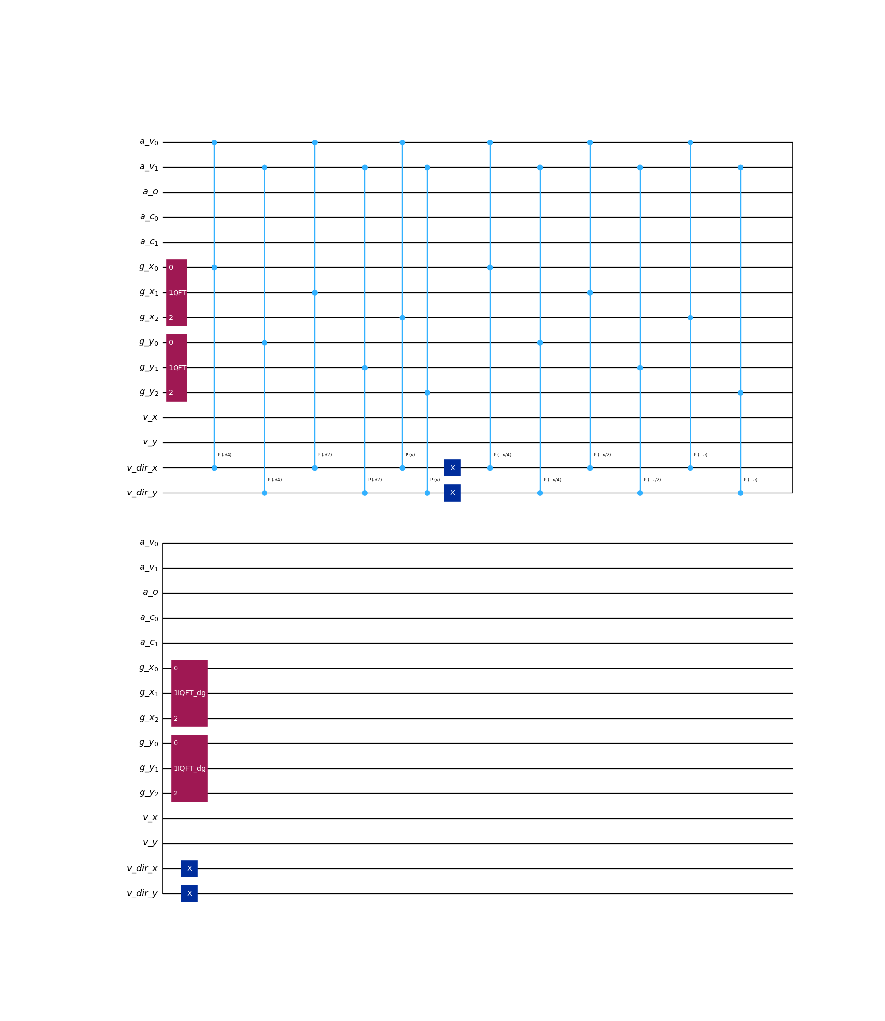

Parameters:

lattice (CollisionlessLattice)
reflection (str | None)
logger (Logger)

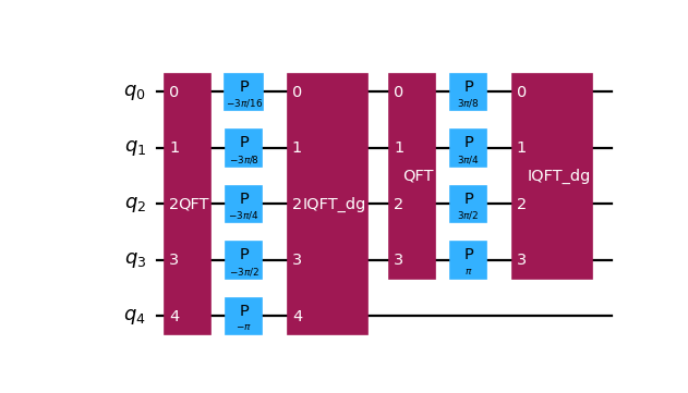
class qlbm.components.collisionless.primitives.SpeedSensitiveAdder(num_qubits, speed, positive, logger=<Logger qlbm (WARNING)>)[source]#

A QFT-based incrementer used to perform streaming in the CQLBM algorithm.

Incrementation and decerementation are performed as rotations on grid qubits that have been previously mapped to the Fourier basis. This happens by nesting a SpeedSensitivePhaseShift primitive between regular and inverse \(QFT\)s.

Attribute	Summary
`num_qubits`	Number of qubits of the circuit.
`speed`	The index of the speed to increment.
`positive`	Whether to increment the particles traveling at this speed in the positive (T) or negative (F) direction.
`logger`	The performance logger, by default getLogger(“qlbm”)

Example usage:

from qlbm.components.collisionless import SpeedSensitiveAdder

SpeedSensitiveAdder(4, 1, True).draw("mpl")

(Source code, png, hires.png, pdf)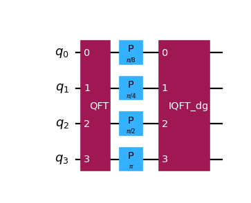

Parameters:

num_qubits (int)
speed (int)
positive (bool)
logger (Logger)

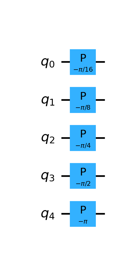
class qlbm.components.collisionless.streaming.SpeedSensitivePhaseShift(num_qubits, speed, positive=False, logger=<Logger qlbm (WARNING)>)[source]#

A primitive that applies the phase-shift as part of the SpeedSensitiveAdder used in Comparators.

The rotation applied is \(\pm \frac{\pi}{2^{n_q - 1 - j}}\), with \(j\) the position of the qubit (indexed starting with 0). Unlike the regular PhaseShift, the speed-sensitive version additionally depends on a specific speed index. For an in-depth mathematical explanation of the procedure, consult Sections 4 and 5.5 of Schalkers and Möller [2].

Attribute	Summary
`num_qubits`	The number of qubits to perform the phase shift for.
`positive`	Whether the phase shift is applied to increment (T) or decrement (F) the position of the particles. Defaults to `False`.
`speed`	The specific speed index to perform the phase shift for.
`logger`	The performance logger, by default `getLogger("qlbm")`.

Example usage:

from qlbm.components.collisionless import SpeedSensitivePhaseShift

# A phase shift of 5 qubits, controlled on speed index 2
SpeedSensitivePhaseShift(num_qubits=5, speed=2, positive=True).draw("mpl")

(Source code, png, hires.png, pdf)

Parameters:

num_qubits (int)
speed (int)
positive (bool)
logger (Logger)

class qlbm.components.collisionless.streaming.PhaseShift(num_qubits, positive=False, logger=<Logger qlbm (WARNING)>)[source]#

A primitive that applies the phase-shift as part of the ControlledIncrementer used in the CollisionlessStreamingOperator.

The rotation applied is \(\pm\frac{\pi}{2^{n_q - 1 - j}}\), with \(j\) the position of the qubit (indexed starting with 0). For an in-depth mathematical explanation of the procedure, consult Section 4 of Schalkers and Möller [2].

Attribute	Summary
`num_qubits`	The number of qubits to perform the phase shift for.
`positive`	Whether the phase shift is applied to increment (T) or decrement (F) the position of the particles. Defaults to `False`.
`logger`	The performance logger, by default `getLogger("qlbm")`.

Example usage:

from qlbm.components.collisionless import PhaseShift

# A phase shift of 5 qubits
PhaseShift(num_qubits=5, positive=False).draw("mpl")

(Source code, png, hires.png, pdf)

Parameters:

num_qubits (int)
positive (bool)
logger (Logger)

Reflection#

class qlbm.components.collisionless.bounceback_reflection.BounceBackReflectionOperator(lattice, blocks, logger=<Logger qlbm (WARNING)>)[source]#

Operator implementing the 2D and 3D Bounce-Back (BB) boundary conditions as described in Schalkers and Möller [3].

The operator parses information encoded in Block objects to detect particles that have virtually streamed into the solid domain before placing them back to their previous positions in the fluid domain. The pseudocode for this procedure is as follows:

Components of the quantum state that encode particles that have streamed inside the obstacle are identified with BounceBackWallComparator objects;
These components have their velocity direction qubits flipped in all three dimensions;
Particles are streamed outside the solid domain with inverted velocity directions;
Once streamed outside the solid domain, components encoding affected particles have their obstacle ancilla qubit reset based on grid position, velocity direction, and whether they have streamed in the CFL timestep.

Attribute	Summary
`lattice`	The `CollisionlessLattice` based on which the properties of the operator are inferred.
`blocks`	A list of `Block` objects for which to generate the BB boundary condition circuits.
`logger`	The performance logger, by default `getLogger("qlbm")`.

Example usage:

from qlbm.components.collisionless import BounceBackReflectionOperator
from qlbm.lattice import CollisionlessLattice

# Build an example lattice
lattice = CollisionlessLattice(
    {
        "lattice": {"dim": {"x": 8, "y": 8}, "velocities": {"x": 4, "y": 4}},
        "geometry": [{"shape":"cuboid", "x": [5, 6], "y": [1, 2], "boundary": "bounceback"}],
    }
)

BounceBackReflectionOperator(lattice=lattice, blocks=lattice.block_list)

(Source code)

Parameters:

lattice (CollisionlessLattice)
blocks (List[Block])
logger (Logger)

create_circuit()[source]#

Creates the qiskit.QuantumCircuit of this object.

This method is called automatically at construction time for all quantum components.

Returns:: The generated QuantumCircuit.
Return type:: QuantumCircuit

reflect_wall(circuit, wall)[source]#

Performs reflection based on information encoded in a ReflectionWall as follows.

A series of \(X\) gates set the grid qubits to the \(\ket{1}\) state for the dimension that the wall spans.
Comparator circuits set the comparator ancilla qubits to \(\ket{1}\) based on the size of the wall in the other dimension(s).
Depending on the use, the directional velocity qubits are also set to \(\ket{1}\) based on the dimension that the wall spans.
A multi-controlled \(X\) gate flips the obstacle ancilla qubit, controlled on the qubits set in the previous steps.
The control qubits are set back to their previous state.

The wall reflection operation is versatile and can be used to both set and re-set the state of the obstacle ancilla qubit at different stages of reflection. When performing BB reflection, this function is first used to flip the ancilla obstacle qubit from \(\ket{0}\) to \(\ket{1}\), irrespective of how particles arrived there. Subsequently, an additional controls are placed on the velocity direction qubits to reset the ancilla obstacle qubit to \(\ket{0}\), after particles have been streamed out of the solid domain.

Parameters:

circuit (QuantumCircuit) – The circuit on which to perform BB reflection of the wall.
wall (ReflectionWall) – The wall encoding the reflection logic.
inside_obstacle (bool) – Whether the wall is inside the obstacle.

Returns:

The circuit performing BB reflection of the wall.

Return type:

QuantumCircuit

reset_edge_state(circuit, edge)[source]#

Resets the state of an edge along the side of an obstacle in 3D as follows.

A series of \(X\) gates set the grid qubits to the \(\ket{1}\) state for the 2 dimensions that the edge spans.
A comparator circuits sets the comparator ancilla qubits to \(\ket{1}\) based on the size of the edge in the remaining dimension.
The directional velocity qubits are also set to \(\ket{1}\) on the specific velocity profile of the targeted particles.
A multi-controlled \(X\) gate flips the obstacle ancilla qubit, controlled on the qubits set in the previous steps.
The control qubits are set back to their previous state.

This function resets the ancilla obstacle qubit to \(\ket{0}\) for particles along 36 specific edges of a cube after those particles have been streamed out of the obstacle in the CFL time step.

Parameters:

circuit (QuantumCircuit) – The circuit on which to perform resetting of the edge state.
edge (ReflectionResetEdge) – The edge on which to apply the reflection reset logic.

Returns:

The circuit performing the resetting of the edge state.

Return type:

QuantumCircuit

reset_point_state(circuit, corner)[source]#

Resets the state of the ancilla obstacle qubit of a single point on the grid as follows.

A series of \(X\) gates set the grid qubits to the \(\ket{1}\) state for the dimension that the wall spans.
The directional velocity qubits are also set to \(\ket{1}\) based on the specific velocity profile of the targeted particles.
A multi-controlled \(X\) gate flips the obstacle ancilla qubit, controlled on the qubits set in the previous steps.
The control qubits are set back to their previous state.

Parameters:

circuit (QuantumCircuit) – The circuit on which to perform the resetting of the point state.
corner (ReflectionPoint) – The corner for which to reset the desired point states.

Returns:

The circuit resetting the point state as desired.

Return type:

QuantumCircuit

flip_and_stream(circuit)[source]#

Flips the velocity direction qubit controlled on the ancilla obstacle qubit, before performing streaming.

Unlike in the regular CollisionlessStreamingOperator, the ControlledIncrementer phase shift circuit is additionally controlled on the ancilla obstacle qubit, which ensures that only particles whose grid position gets incremented (decremented) are those that have streamed inside the solid domain in this CFL time step.

Parameters:: circuit (QuantumCircuit) – The circuit on which to perform the flip and stream operation.

class qlbm.components.collisionless.specular_reflection.SpecularReflectionOperator(lattice, blocks, logger=<Logger qlbm (WARNING)>)[source]#

Operator implementing the 2D and 3D Specular Reflection (SR) boundary conditions as described Schalkers and Möller [2].

The operator parses information encoded in Block objects to detect particles that have virtually streamed into the solid domain before placing them back to their previous positions in the fluid domain. The pseudocode for this procedure is as follows:

Components of the quantum state that encode particles that have streamed inside the obstacle are identified with SpecularWallComparator objects;
These components have their velocity direction qubits flipped according to the wall they came in contact with. Where two or three walls come together, the two or three corresponding directions are inverted;
Particles are streamed outside the solid domain with inverted velocity directions;
Once streamed outside the solid domain, components encoding affected particles have their obstacle ancilla qubits reset based on grid position, velocity direction, and whether they have streamed in the CFL timestep.

Attribute	Summary
`lattice`	The `CollisionlessLattice` based on which the properties of the operator are inferred.
`blocks`	A list of `Block` objects for which to generate the BB boundary condition circuits.
`logger`	The performance logger, by default `getLogger("qlbm")`.

Example usage:

from qlbm.components.collisionless import SpecularReflectionOperator
from qlbm.lattice import CollisionlessLattice

# Build an example lattice
lattice = CollisionlessLattice(
    {
        "lattice": {"dim": {"x": 8, "y": 8}, "velocities": {"x": 4, "y": 4}},
        "geometry": [{"shape":"cuboid", "x": [5, 6], "y": [1, 2], "boundary": "specular"}],
    }
)

SpecularReflectionOperator(lattice=lattice, blocks=lattice.block_list)

(Source code)

Parameters:

lattice (CollisionlessLattice)
blocks (List[Block])
logger (Logger)

create_circuit()[source]#

Creates the qiskit.QuantumCircuit of this object.

This method is called automatically at construction time for all quantum components.

Returns:: The generated QuantumCircuit.
Return type:: QuantumCircuit

reflect_wall(circuit, wall)[source]#

Performs reflection based on information encoded in a ReflectionWall as follows.

A series of \(X\) gates set the grid qubits to the \(\ket{1}\) state for the dimension that the wall spans.
Comparator circuits set the comparator ancilla qubits to \(\ket{1}\) based on the size of the wall in the other dimension(s).
Depending on the use, the directional velocity qubits are also set to \(\ket{1}\) based on the dimension that the wall spans.
A multi-controlled \(X\) gate flips the obstacle ancilla qubits of the particular dimension that the wall reflects, controlled on the qubits set in the previous steps.
The control qubits are set back to their previous state.

The wall reflection operation is versatile and can be used to both set and re-set the state of the obstacle ancilla qubit at different stages of reflection. When performing SR reflection, this function is first used to flip the ancilla obstacle qubit from \(\ket{0}\) to \(\ket{1}\), irrespective of how particles arrived there. Subsequently, an additional controls are placed on the velocity direction qubits to reset the ancilla obstacle qubit to \(\ket{0}\), after particles have been streamed out of the solid domain.

Parameters:

circuit (QuantumCircuit) – The circuit on which to perform resetting of the edge state.
wall (ReflectionWall) – The wall encoding the reflection logic.

Returns:

The circuit performing specular reflection of the wall.

Return type:

QuantumCircuit

reset_edge_state(circuit, edge)[source]#

Resets the state of an edge along the side of an obstacle in 3D as follows.

A series of \(X\) gates set the grid qubits to the \(\ket{1}\) state for the 2 dimensions that the edge spans.
A comparator circuits sets the comparator ancilla qubits to \(\ket{1}\) based on the size of the edge in the remaining dimension.
The directional velocity qubits are also set to \(\ket{1}\) on the specific velocity profile of the targeted particles.
A multi-controlled \(X\) gate flips the obstacle ancilla qubits of the direction reflect by the wall(s) that the edge is next to, controlled on the qubits set in the previous steps.
The control qubits are set back to their previous state.

This function resets the ancilla obstacle qubit to \(\ket{0}\) for particles along 36 specific edges of a cube after those particles have been streamed out of the obstacle in the CFL time step.

Parameters:

circuit (QuantumCircuit) – The circuit on which to perform resetting of the edge state.
edge (ReflectionResetEdge) – The edge on which to apply the reflection reset logic.

Returns:

The circuit performing the resetting of the edge state.

Return type:

QuantumCircuit

reset_point_state(circuit, corner)[source]#

Resets the state of the ancilla obstacle qubit of a single point on the grid as follows.

A series of \(X\) gates set the grid qubits to the \(\ket{1}\) state for the dimension that the wall spans.
The directional velocity qubits are also set to \(\ket{1}\) based on the specific velocity profile of the targeted particles.
A multi-controlled \(X\) gate flips the obstacle ancilla qubits corresponding to the dimensions that particles would have traveled to arrive there via reflection, controlled on the qubits set in the previous steps.
The control qubits are set back to their previous state.

Parameters:

circuit (QuantumCircuit) – The circuit on which to perform the resetting of the point state.
corner (ReflectionPoint) – The corner for which to reset the desired point states.

Returns:

The circuit resetting the point state as desired.

Return type:

QuantumCircuit

flip_and_stream(circuit)[source]#

Flips the velocity direction qubit controlled on the ancilla obstacle qubit, before performing streaming.

Unlike in the regular CollisionlessStreamingOperator, the ControlledIncrementer phase shift circuit is additionally controlled on the ancilla obstacle qubit of the streaming dimension, which ensures that only particles whose grid position gets incremented (decremented) are those that have streamed inside the solid domain in this CFL time step.

Parameters:: circuit (QuantumCircuit) – The circuit on which to perform the flip and stream operation.

class qlbm.components.collisionless.bounceback_reflection.BounceBackWallComparator(lattice, wall, logger=<Logger qlbm (WARNING)>)[source]#

A primitive used in the collision BounceBackReflectionOperator that implements the comparator for the BB boundary conditions as described in Schalkers and Möller [3].

The comparator sets an ancilla qubit to \(\ket{1}\) for the components of the quantum state whose grid qubits fall within the range spanned by the wall.

Attribute	Summary
`lattice`	The `CollisionlessLattice` based on which the properties of the operator are inferred.
`wall`	The `ReflectionWall` encoding the range spanned by the wall.
`logger`	The performance logger, by default `getLogger("qlbm")`.

Example usage:

from qlbm.components.collisionless import BounceBackWallComparator
from qlbm.lattice import CollisionlessLattice

# Build an example lattice
lattice = CollisionlessLattice(
    {
        "lattice": {"dim": {"x": 8, "y": 8}, "velocities": {"x": 4, "y": 4}},
        "geometry": [{"shape":"cuboid", "x": [5, 6], "y": [1, 2], "boundary": "bounceback"}],
    }
)

# Comparing on the indices of the inside x-wall on the lower-bound of the obstacle
BounceBackWallComparator(
    lattice=lattice, wall=lattice.block_list[0].walls_inside[0][0]
).draw("mpl")

(Source code, png, hires.png, pdf)

Parameters:

lattice (CollisionlessLattice)
wall (ReflectionWall)
logger (Logger)

class qlbm.components.collisionless.specular_reflection.SpecularWallComparator(lattice, wall, logger=<Logger qlbm (WARNING)>)[source]#

A primitive used in the collisionless SpecularReflectionOperator that implements the comparator for the specular reflection boundary conditions around the wall as described Schalkers and Möller [2].

The comparator sets the d ancilla qubits to \(\ket{1}\) for the components of the quantum state whose grid qubits fall within the range spanned by the wall.

Attribute	Summary
`lattice`	The `CollisionlessLattice` based on which the properties of the operator are inferred.
`wall`	The `ReflectionWall` encoding the range spanned by the wall.
`logger`	The performance logger, by default `getLogger("qlbm")`.

Example usage:

from qlbm.components.collisionless import SpecularWallComparator
from qlbm.lattice import CollisionlessLattice

# Build an example lattice
lattice = CollisionlessLattice(
    {
        "lattice": {"dim": {"x": 8, "y": 8}, "velocities": {"x": 4, "y": 4}},
        "geometry": [{"shape":"cuboid", "x": [5, 6], "y": [1, 2], "boundary": "specular"}],
    }
)

# Comparing on the indices of the inside x-wall on the lower-bound of the obstacle
SpecularWallComparator(
    lattice=lattice, wall=lattice.block_list[0].walls_inside[0][0]
).draw("mpl")

(Source code, png, hires.png, pdf)

Parameters:

lattice (CollisionlessLattice)
wall (ReflectionWall)
logger (Logger)

class qlbm.components.collisionless.primitives.EdgeComparator(lattice, edge, logger=<Logger qlbm (WARNING)>)[source]#

A primitive used in the 3D collisionless SpecularReflectionOperator and BounceBackReflectionOperator described in Schalkers and Möller [2].

Attribute	Summary
`lattice`	The `CollisionlessLattice` based on which the properties of the operator are inferred.
`logger`	The performance logger, by default `getLogger("qlbm")`.
`edge`	The coordinates of the edge within the grid.

Example usage:

from qlbm.components.collisionless import EdgeComparator
from qlbm.lattice import CollisionlessLattice

# Build an example lattice
lattice = CollisionlessLattice(
    {
        "lattice": {
            "dim": {"x": 8, "y": 8, "z": 8},
            "velocities": {"x": 4, "y": 4, "z": 4},
        },
        "geometry": [{"shape":"cuboid", "x": [2, 5], "y": [2, 5], "z": [2, 5], "boundary": "specular"}],
    }
)

# Draw the edge comparator circuit for one specific corner edge
EdgeComparator(lattice, lattice.block_list[0].corner_edges_3d[0]).draw("mpl")

(Source code, png, hires.png, pdf)

Parameters:

lattice (CollisionlessLattice)
edge (ReflectionResetEdge)
logger (Logger)

class qlbm.components.collisionless.primitives.Comparator(num_qubits, num_to_compare, mode, logger=<Logger qlbm (WARNING)>)[source]#

Quantum comparator primitive that compares two a quantum state of num_qubits qubits and an integer num_to_compare with respect to a ComparatorMode.

Attribute	Summary
`num_qubits`	Number of qubits encoding the integer to compare.
`num_to_compare`	The integer to compare against.
`mode`	The `ComparatorMode` used to compare the two numbers.
`logger`	The performance logger, by default getLogger(“qlbm”)

Example usage:

from qlbm.components.collisionless import Comparator, ComparatorMode

# On a 5 qubit register, compare the number 3
Comparator(num_qubits=5,
           num_to_compare=3,
           mode=ComparatorMode.LT).draw("mpl")

(Source code, png, hires.png, pdf)

Parameters:

num_qubits (int)
num_to_compare (int)
mode (ComparatorMode)
logger (Logger)

class qlbm.components.collisionless.primitives.ComparatorMode(value, names=<not given>, *values, module=None, qualname=None, type=None, start=1, boundary=None)[source]#

Enumerator for the modes of quantum comparator circuits.

The modes are as follows:

(1, ComparatorMode.LT, \(<\));
(2, ComparatorMode.LE, \(\leq\));
(3, ComparatorMode.GT, \(>\));
(4, ComparatorMode.GE, \(\geq\)).

Others#

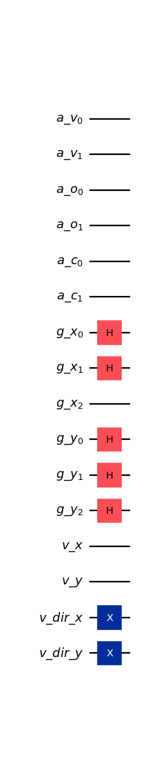
class qlbm.components.collisionless.primitives.CollisionlessInitialConditions(lattice, logger=<Logger qlbm (WARNING)>)[source]#

A primitive that creates the quantum circuit to prepare the flow field in its initial conditions.

The initial conditions create a quantum state spanning half the grid in the x-axis, and the entirety of the y (and z)-axes (if 3D). All velocities are pointing in the positive direction.

Attribute	Summary
`lattice`	The `CollisionlessLattice` based on which the properties of the operator are inferred.
`logger`	The performance logger, by default `getLogger("qlbm")`.

Example usage:

from qlbm.components.collisionless import CollisionlessInitialConditions
from qlbm.lattice import CollisionlessLattice

# Build an example lattice
lattice = CollisionlessLattice({
    "lattice": {
        "dim": {
                "x": 8,
                "y": 8
            },
            "velocities": {
                "x": 4,
                "y": 4
        }
    },
    "geometry": [
        {
            "shape": "cuboid",
            "x": [5, 6],
            "y": [1, 2],
            "boundary": "specular"
        }
    ]
})

# Draw the initial conditions circuit
CollisionlessInitialConditions(lattice).draw("mpl")

(Source code, png, hires.png, pdf)

Parameters:

lattice (CollisionlessLattice)
logger (Logger)

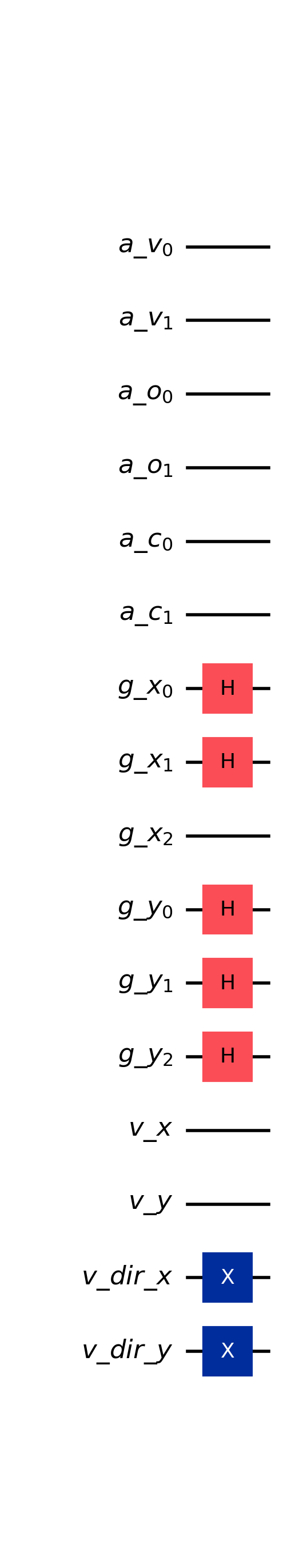
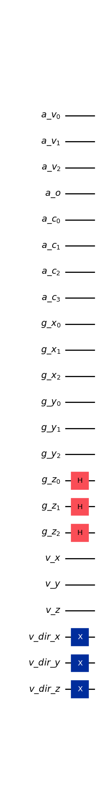
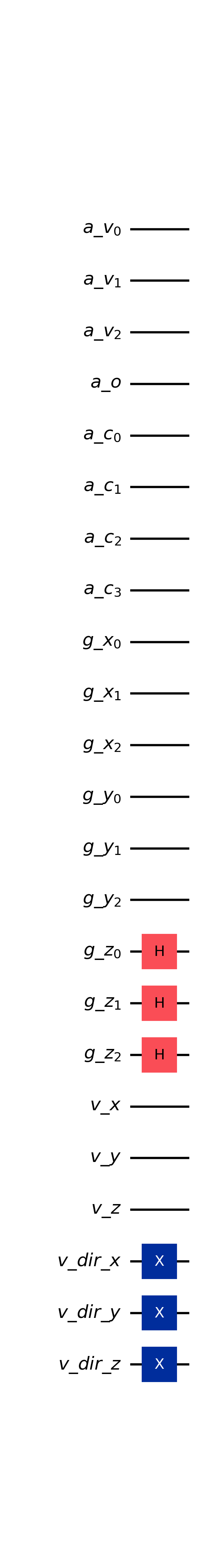
class qlbm.components.collisionless.primitives.CollisionlessInitialConditions3DSlim(lattice, logger=<Logger qlbm (WARNING)>)[source]#

A primitive that creates the quantum circuit to prepare the flow field in its initial conditions for 3 dimensions.

The initial conditions create the quantum state \(\Sigma_{j}\ket{0}^{\otimes n_{g_x}}\ket{0}^{\otimes n_{g_y}}\ket{j}\) over the grid qubits, that is, spanning the z-axis at the bottom of the x- and y-axes. This is helpful for debugging edge cases around the corners of 3D obstacles. All velocities are pointing in the positive direction.

Attribute	Summary
`lattice`	The `CollisionlessLattice` based on which the properties of the operator are inferred.
`logger`	The performance logger, by default `getLogger("qlbm")`.

Example usage:

from qlbm.components.collisionless import CollisionlessInitialConditions3DSlim
from qlbm.lattice import CollisionlessLattice

# Build an example lattice
lattice = CollisionlessLattice({
    "lattice": {
        "dim": {
        "x": 8,
        "y": 8,
        "z": 8
        },
        "velocities": {
        "x": 4,
        "y": 4,
        "z": 4
        }
    },
    "geometry": []
})

# Draw the initial conditions circuit
CollisionlessInitialConditions3DSlim(lattice).draw("mpl")

(Source code, png, hires.png, pdf)

Parameters:

lattice (CollisionlessLattice)
logger (Logger)

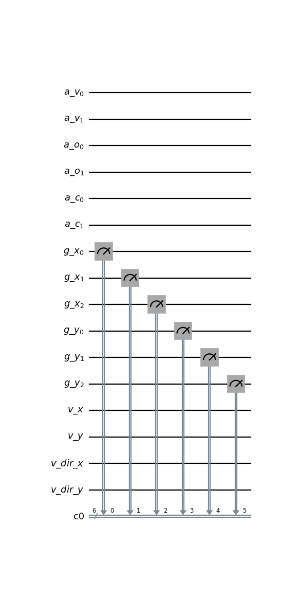
class qlbm.components.collisionless.primitives.GridMeasurement(lattice, logger=<Logger qlbm (WARNING)>)[source]#

A primitive that implements a measurement operation on the grid qubits.

Used at the end of the time step circuit to extract information from the quantum state.

Attribute	Summary
`lattice`	The `CollisionlessLattice` based on which the properties of the operator are inferred.
`logger`	The performance logger, by default `getLogger("qlbm")`.

Example usage:

from qlbm.components.collisionless import GridMeasurement
from qlbm.lattice import CollisionlessLattice

# Build an example lattice
lattice = CollisionlessLattice({
    "lattice": {
        "dim": {
                "x": 8,
                "y": 8
            },
            "velocities": {
                "x": 4,
                "y": 4
        }
    },
    "geometry": [
        {
            "shape": "cuboid",
            "x": [5, 6],
            "y": [1, 2],
            "boundary": "specular"
        }
    ]
})

# Draw the measurement circuit
GridMeasurement(lattice).draw("mpl")

(Source code, png, hires.png, pdf)

Parameters:

lattice (CollisionlessLattice)
logger (Logger)

Collisionless Circuits#

End-to-end algorithms#

Streaming#

Reflection#

Others#

This Page