Space-Time Circuits#
This page contains documentation about the quantum circuits that make up the Space-Time Quantum Lattice Boltzmann Method (STQLBM) described in [4]. At its core, the Space-Time QLBM uses an extended computational basis state encoding that that circumvents the non-locality of the streaming step by including additional information from neighboring grid points. This happens in several distinct steps:
Initial conditions prepare the starting state of the probability distribution function.
Streaming moves the position of particles to neighboring points according to their velocity.
Collision locally changes the velocity profile of particles positioned at the same position in space.
Measurement operations extract information out of the quantum state, which can later be post-processed classically.
This page documents the individual components that make up the STQLBM algorithm. Subsections follow a top-down approach, where end-to-end operators are introduced first, before being broken down into their constituent parts.
Warning
The STQBLM algorithm is a based on typical \(D_dQ_q\) discretizations.
The current implementation only supports \(D_2Q_4\) for one time step.
This is work in progress.
Multiple steps are possible through qlbm‘s reinitialization mechanism.
End-to-end algorithms#
- class qlbm.components.spacetime.spacetime.SpaceTimeQLBM(lattice, filter_inside_blocks=True, logger=<Logger qlbm (WARNING)>)[source]#
The end-to-end algorithm of the Space-Time Quantum Lattice Boltzmann Algorithm described in [4].
This implementation currently only supports 1 time step on the \(D_2Q_4\) lattice discretization. Additional steps are possible by means of reinitialization.
The algorithm is composed of two main steps, the implementation of which (in general) varies per individual time step:
Streaming performed by the
SpaceTimeStreamingOperatormoves the particles on the grid by means of swap gates over velocity qubits.Collision performed by the
SpaceTimeCollisionOperatordoes not move particles on the grid, but locally alters the velocity qubits at each grid point, if applicable.
Attribute
Summary
latticeThe
SpaceTimeLatticebased on which the properties of the operator are inferred.loggerThe performance logger, by default
getLogger("qlbm").Example usage:
from qlbm.components.spacetime import SpaceTimeQLBM
from qlbm.lattice import SpaceTimeLattice

# Build an example lattice
lattice = SpaceTimeLattice(
    num_timesteps=1,
    lattice_data={
        "lattice": {"dim": {"x": 4, "y": 8}, "velocities": {"x": 2, "y": 2}},
        "geometry": [],
    },
)

# Draw the end-to-end algorithm for 1 time step
SpaceTimeQLBM(lattice=lattice).draw("mpl")
(
Source code,png,hires.png,pdf)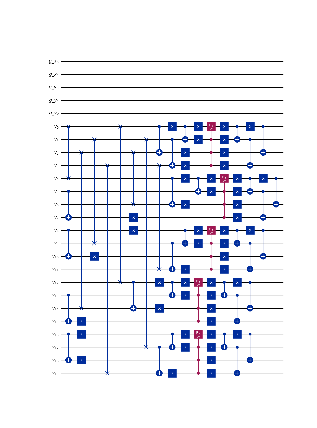
- Parameters:
lattice (SpaceTimeLattice)
filter_inside_blocks (bool)
logger (Logger)
Streaming#
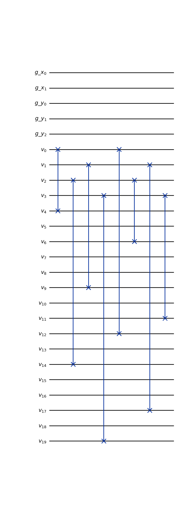
- class qlbm.components.spacetime.streaming.SpaceTimeStreamingOperator(lattice, timestep, logger=<Logger qlbm (WARNING)>)[source]#
An operator that performs streaming as a series of \(SWAP\) gates as part of the
SpaceTimeQLBMalgorithm.The velocities corresponding to neighboring gridpoints are streamed “into” the gridpoint affected relative to the
timestep. The register setup of theSpaceTimeLatticeis such that following each time step, an additional “layer” neighboring velocity qubits can be discarded, since the information they encode can never reach the relative origin in the remaining number of time steps. As such, the complexity of the streaming operator decreases with the number of steps (still) to be simulated. For an in-depth mathematical explanation of the procedure, consult pages 15-18 of Schalkers and Möller [4].Attribute
Summary
latticeThe
SpaceTimeLatticebased on which the properties of the operator are inferred.timestepThe time step for which to perform streaming.
loggerThe performance logger, by default
getLogger("qlbm").Example usage:
from qlbm.components.spacetime import SpaceTimeStreamingOperator
from qlbm.lattice import SpaceTimeLattice

# Build an example lattice
lattice = SpaceTimeLattice(
    num_timesteps=1,
    lattice_data={
        "lattice": {"dim": {"x": 4, "y": 8}, "velocities": {"x": 2, "y": 2}},
        "geometry": [],
    },
)

# Draw the streaming operator for 1 time step
SpaceTimeStreamingOperator(lattice=lattice, timestep=1).draw("mpl")
(
Source code,png,hires.png,pdf)
- Parameters:
lattice (SpaceTimeLattice)
timestep (int)
logger (Logger)
Collision#
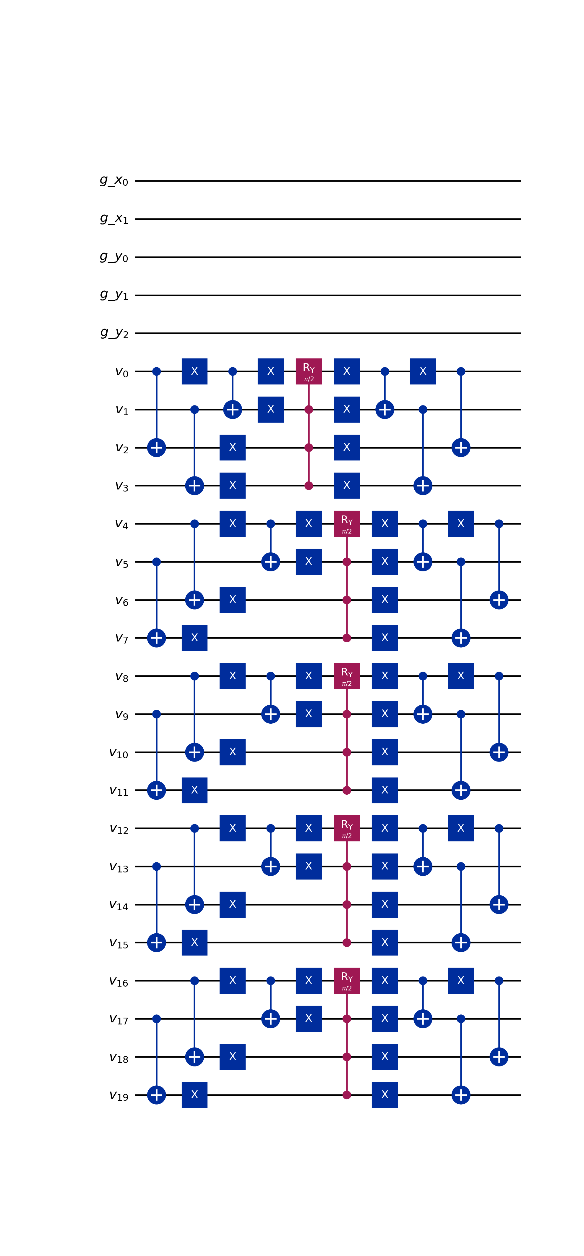
- class qlbm.components.spacetime.collision.SpaceTimeCollisionOperator(lattice, timestep, gate_to_apply=Instruction(name='ry', num_qubits=1, num_clbits=0, params=[1.5707963267948966]), logger=<Logger qlbm (WARNING)>)[source]#
An operator that performs collision part of the
SpaceTimeQLBMalgorithm.Collision is a local operation that is performed simultaneously on all velocity qubits corresponding to a grid location. In practice, this means the same circuit is repeated across all “local” qubit register chunks. Collision can be understood as follows:
For each group of qubits, the states encoding velocities belonging to a particular equivalence class are first isolated with a series of \(X\) and \(CX\) gates. This leaves qubits not affected by the rotation in \(\ket{1}^{\otimes n_v-1}\) state.
A rotation gate is applied to the qubit(s) relevant to the equivalence class shift, controlled on the qubits set in the previous step.
The operation performed in Step 1 is undone.
The register setup of the
SpaceTimeLatticeis such that following each time step, an additional “layer” neighboring velocity qubits can be discarded, since the information they encode can never reach the relative origin in the remaining number of time steps. As such, the complexity of the collision operator decreases with the number of steps (still) to be simulated. For an in-depth mathematical explanation of the procedure, consult pages 11-15 of Schalkers and Möller [4].Attribute
Summary
latticeThe
SpaceTimeLatticebased on which the properties of the operator are inferred.timestepThe time step for which to perform streaming.
gate_to_applyThe gate to apply to the velocities matching equivalence classes. Defaults to \(R_y(\frac{\pi}{2})\).
loggerThe performance logger, by default
getLogger("qlbm").Example usage:
from qlbm.components.spacetime import SpaceTimeCollisionOperator
from qlbm.lattice import SpaceTimeLattice

# Build an example lattice
lattice = SpaceTimeLattice(
    num_timesteps=1,
    lattice_data={
        "lattice": {"dim": {"x": 4, "y": 8}, "velocities": {"x": 2, "y": 2}},
        "geometry": [],
    },
)

# Draw the collision operator for 1 time step
SpaceTimeCollisionOperator(lattice=lattice, timestep=1).draw("mpl")
(
Source code,png,hires.png,pdf)
- Parameters:
lattice (SpaceTimeLattice)
timestep (int)
gate_to_apply (Gate)
logger (Logger)
Others#
- class qlbm.components.spacetime.initial.PointWiseSpaceTimeInitialConditions(lattice, grid_data=[((2, 5), (True, True, True, True)), ((3, 4), (False, True, False, True))], filter_inside_blocks=True, logger=<Logger qlbm (WARNING)>)[source]#
Prepares the initial state for the
SpaceTimeQLBM.Initial conditions are supplied in a
List[Tuple[Tuple[int, int], Tuple[bool, bool, bool, bool]]]containing, for each population to be initialized, two nested tuples.The first tuple position of the population(s) on the grid (i.e.,
(2, 5)). The second tuple contains velocity of the population(s) at that location. Since the maximum number of velocities is pre-determined and the computational basis state encoding favors boolean logic, the input is provided as a tuple ofbooleans. That is,(True, True, False, False)would mean there are two populations at the same gridpoint, with velocities \(q_0\) and \(q_1\) according to the \(D_2Q_4\) discretization. Together, thegrid_dataargument of the constructor can be supplied as, for instance,[((3, 7), (False, True, False, True))].The initialization follows the following steps:
- For each (position, velocity) pair:
Set the gird qubits encoding the position to \(\ket{1}^{\otimes n_g}\) using \(X\) gates;
Set each of the toggled velocities to \(\ket{1}\) by means of \(MCX\) gates, controlled on the qubits set in the previous step;
Undo the operation of step 1 (i.e., repeat the \(X\) gates);
Repeat steps 1-3 for all neighboring velocity qubits, adjusting for grid position and relative velocity index.
Attribute
Summary
grid_dataThe information encoding the particle probability distribution, formatted as (position, velocity) tuples.
latticeThe
SpaceTimeLatticebased on which the properties of the operator are inferred.loggerThe performance logger, by default
getLogger("qlbm").Example usage:
from qlbm.components.spacetime.initial import PointWiseSpaceTimeInitialConditions
from qlbm.lattice import SpaceTimeLattice

# Build an example lattice
lattice = SpaceTimeLattice(
    num_timesteps=1,
    lattice_data={
        "lattice": {"dim": {"x": 4, "y": 8}, "velocities": {"x": 2, "y": 2}},
        "geometry": [],
    },
)

# Draw the initial conditions for two particles at (3, 7), traveling in the +y and -y directions
PointWiseSpaceTimeInitialConditions(lattice=lattice, grid_data=[((3, 7), (False, True, False, True))]).draw("mpl")
(
Source code,png,hires.png,pdf)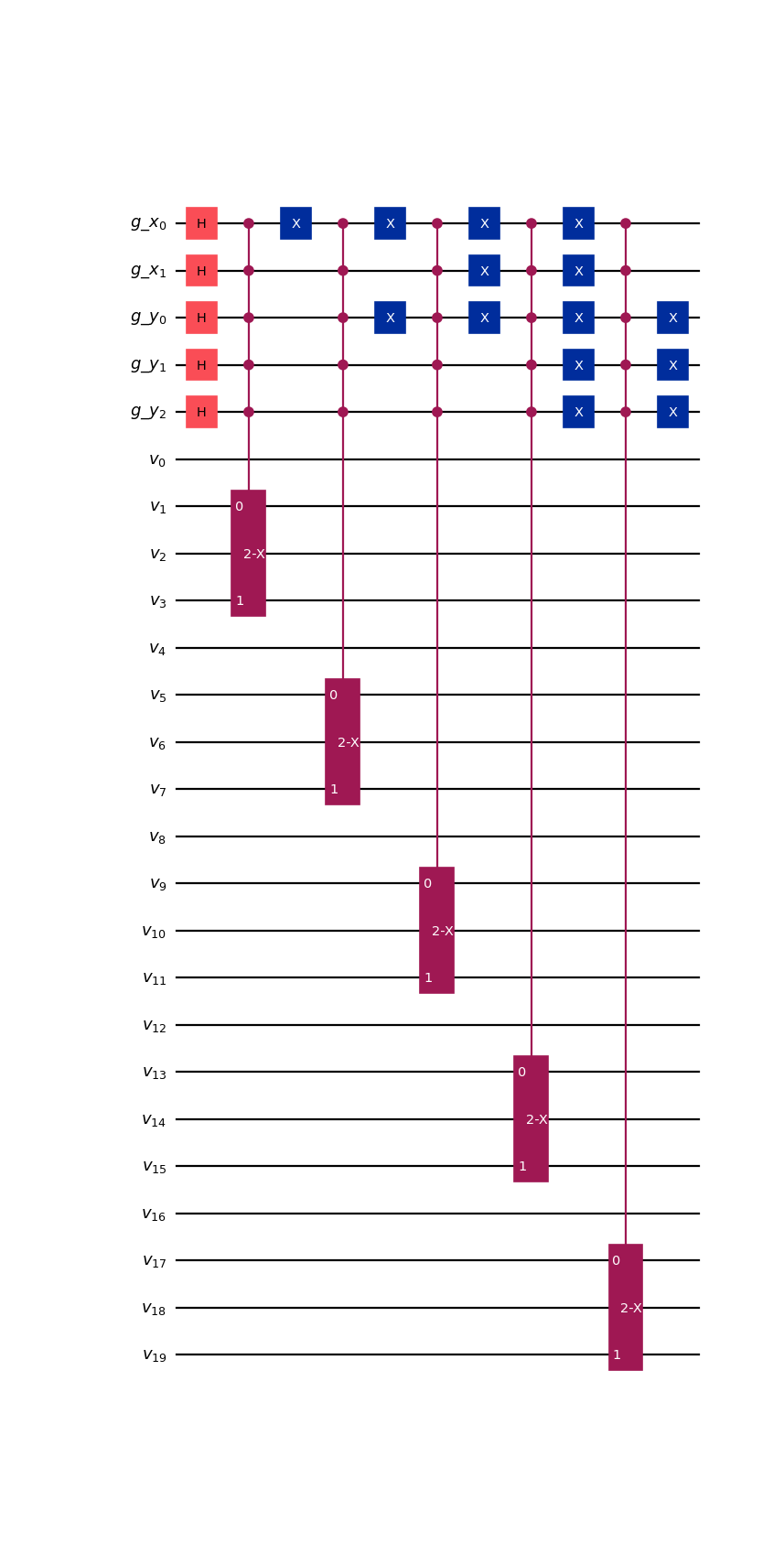
- Parameters:
lattice (SpaceTimeLattice)
grid_data (List[Tuple[Tuple[int, ...], Tuple[bool, ...]]])
filter_inside_blocks (bool)
logger (Logger)
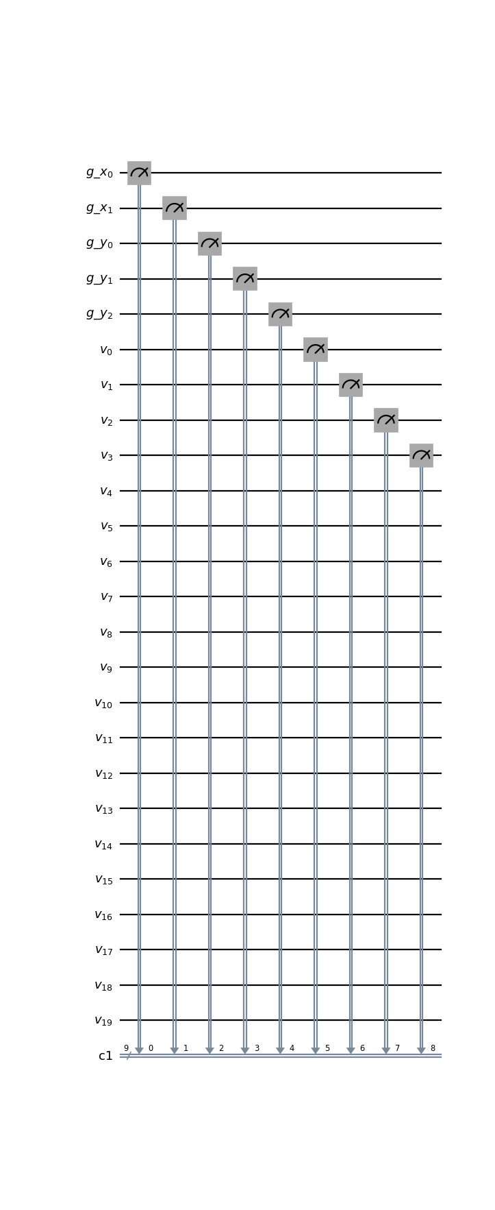
- class qlbm.components.spacetime.measurement.SpaceTimeGridVelocityMeasurement(lattice, logger=<Logger qlbm (WARNING)>)[source]#
A primitive that implements a measurement operation on the grid and the local velocity qubits.
Used at the end of the simulation to extract information from the quantum state. Together, the information from the local and grid qubits can be used for on-the-fly reinitialization.
Attribute
Summary
latticeThe
SpaceTimeLatticebased on which the properties of the operator are inferred.loggerThe performance logger, by default
getLogger("qlbm").Example usage:
from qlbm.components.spacetime import SpaceTimeGridVelocityMeasurement
from qlbm.lattice import SpaceTimeLattice

# Build an example lattice
lattice = SpaceTimeLattice(
    num_timesteps=1,
    lattice_data={
        "lattice": {"dim": {"x": 4, "y": 8}, "velocities": {"x": 2, "y": 2}},
        "geometry": [],
    },
)

# Draw the measurement circuit
SpaceTimeGridVelocityMeasurement(lattice=lattice).draw("mpl")
(
Source code,png,hires.png,pdf)
- Parameters:
lattice (SpaceTimeLattice)
logger (Logger)